Separate mother and teacher RI-CLPM for social isolation and ADHD symptoms in childhood
dat.raw <- read_dta(paste0(data.raw_path, "Katie_19Jan22.dta"))

dat <- dat.raw %>%
  dplyr::select(id = atwinid,
         sampsex,
         seswq35,
         sisoem5,  # social isolation mother report
         sisoem7,
         sisoem10,
         sisoem12,
         sisoet5,  # social isolation teacher report
         sisoet7,
         sisoet10,
         sisoet12,
         tadhdem5,  # total ADHD mother report
         tadhdem7,
         tadhdem10,
         tadhdem12,
         tadhdet5,  # total ADHD teacher report
         tadhdet7,
         tadhdet10,
         tadhdet12,
         hyem5,     # hyperactivity ADHD mother report
         hyem7,
         hyem10,
         hyem12,
         hyet5,     # hyperactivity ADHD teacher report
         hyet7,
         hyet10,
         hyet12,
         inem5,    # inattention ADHD mother report
         inem7,
         inem10,
         inem12,
         inet5,    # inattention ADHD teacher report
         inet7,
         inet10,
         inet12,
         sisoe5,
         sisoe7,
         sisoe10,
         sisoe12
  )

colnames(dat)
[1] “id” “sampsex” “seswq35” “sisoem5” “sisoem7” “sisoem10” [7] “sisoem12” “sisoet5” “sisoet7” “sisoet10” “sisoet12” “tadhdem5” [13] “tadhdem7” “tadhdem10” “tadhdem12” “tadhdet5” “tadhdet7” “tadhdet10” [19] “tadhdet12” “hyem5” “hyem7” “hyem10” “hyem12” “hyet5”
[25] “hyet7” “hyet10” “hyet12” “inem5” “inem7” “inem10”
[31] “inem12” “inet5” “inet7” “inet10” “inet12” “sisoe5”
[37] “sisoe7” “sisoe10” “sisoe12”
Functions
# Table of model fit
table.model.fit <- function(model){
  model.fit <- as.data.frame(t(as.data.frame(model$FIT))) %>%
    dplyr::select(chisq, df, chisq.scaled, cfi.robust, tli.robust, aic, bic, bic2, rmsea.robust, rmsea.ci.lower.robust, rmsea.ci.upper.robust, srmr) #can only be used with "MLR" estimator
  return(model.fit)
}

# Table of regression and correlation (standardised covariance) coefficients
table.model.coef <- function(model, type, constraints){
  if (type == "RICLPM" & constraints == "No"){
    model.coef <- as.tibble(model$PE[c(17:32),]) %>% dplyr::select(-exo, -std.lv, -std.nox)
    return(model.coef)
  } else if(type == "RICLPM" & constraints == "Yes"){
    model.coef <- as.tibble(model$PE[c(17:32),]) %>% dplyr::select(-exo, -label, -std.lv, -std.nox)
    return(model.coef)
  } else if(type == "CLPM" & constraints == "No"){
    model.coef <- as.tibble(model$PE[c(1:16),]) %>% dplyr::select(-exo, -std.lv, -std.nox)
    return(model.coef)
  } else if(type == "CLPM" & constraints == "Yes"){
    model.coef <- as.tibble(model$PE[c(1:16),]) %>% dplyr::select(-exo, -std.lv, -std.nox)
    return(model.coef)
  } else {model.coef <- NULL}
}
Normality checks
If the data is non-normal - we should use robust test statistics for all models going forward. Robust standard errors will also be calculated to account for the use of twins in our sample.
# mother
hist(dat$sisoem5)
hist(dat$sisoem7)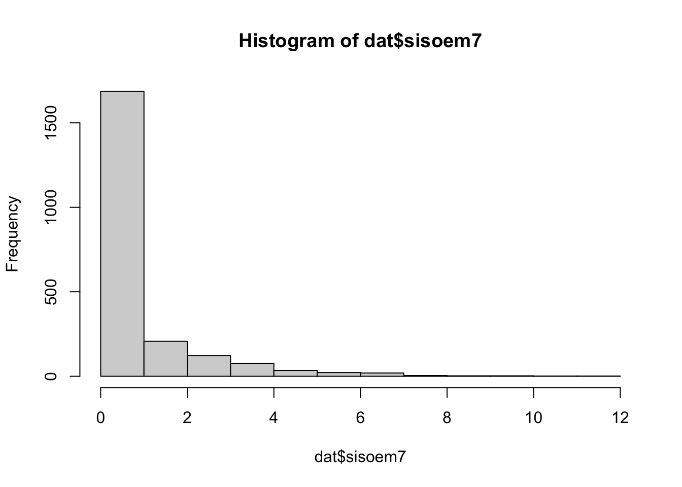
hist(dat$sisoem10)
hist(dat$sisoem12)
# teacher
hist(dat$sisoet5)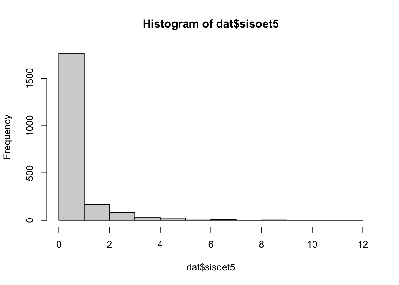
hist(dat$sisoet7)
hist(dat$sisoet10)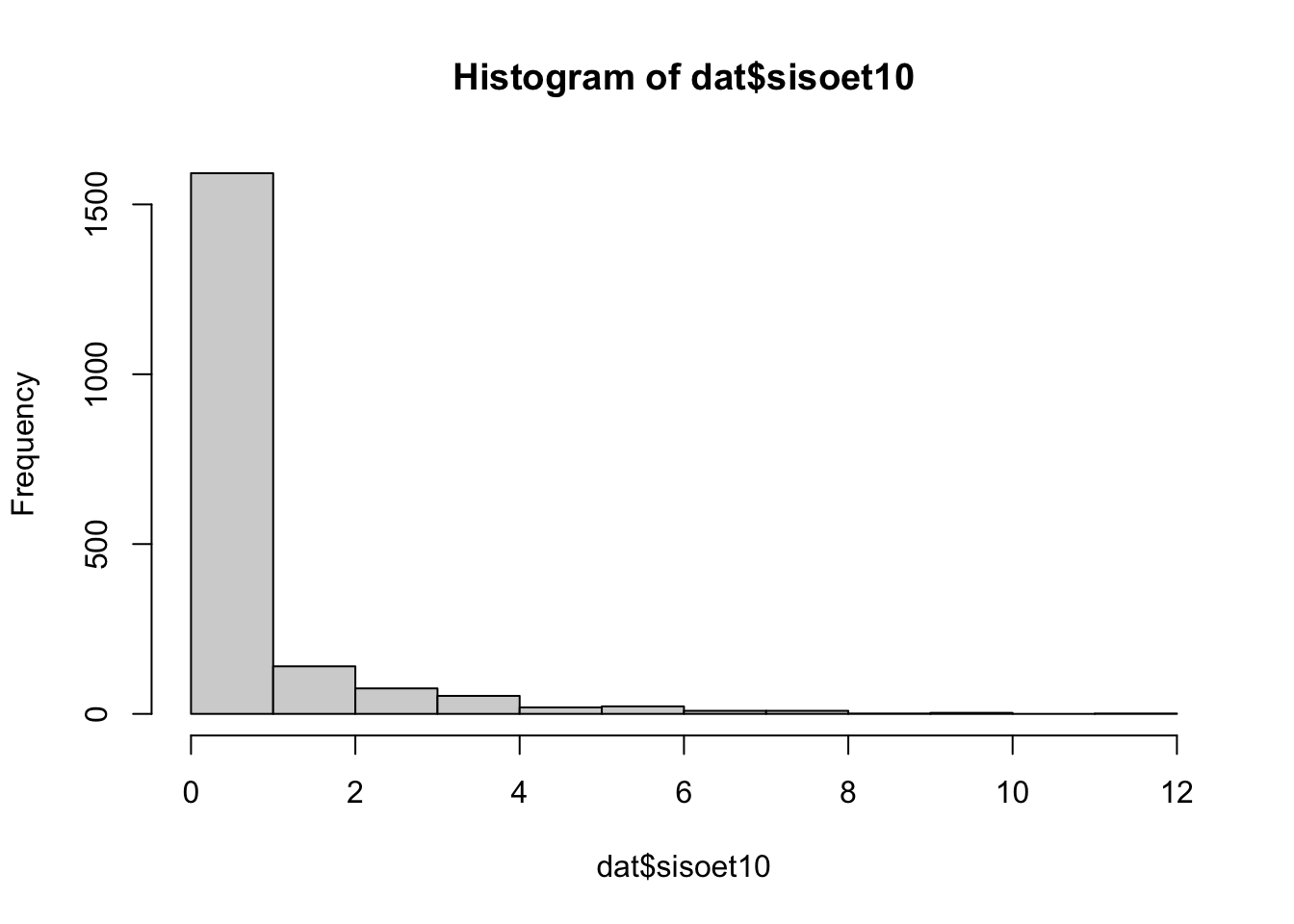
hist(dat$sisoet12)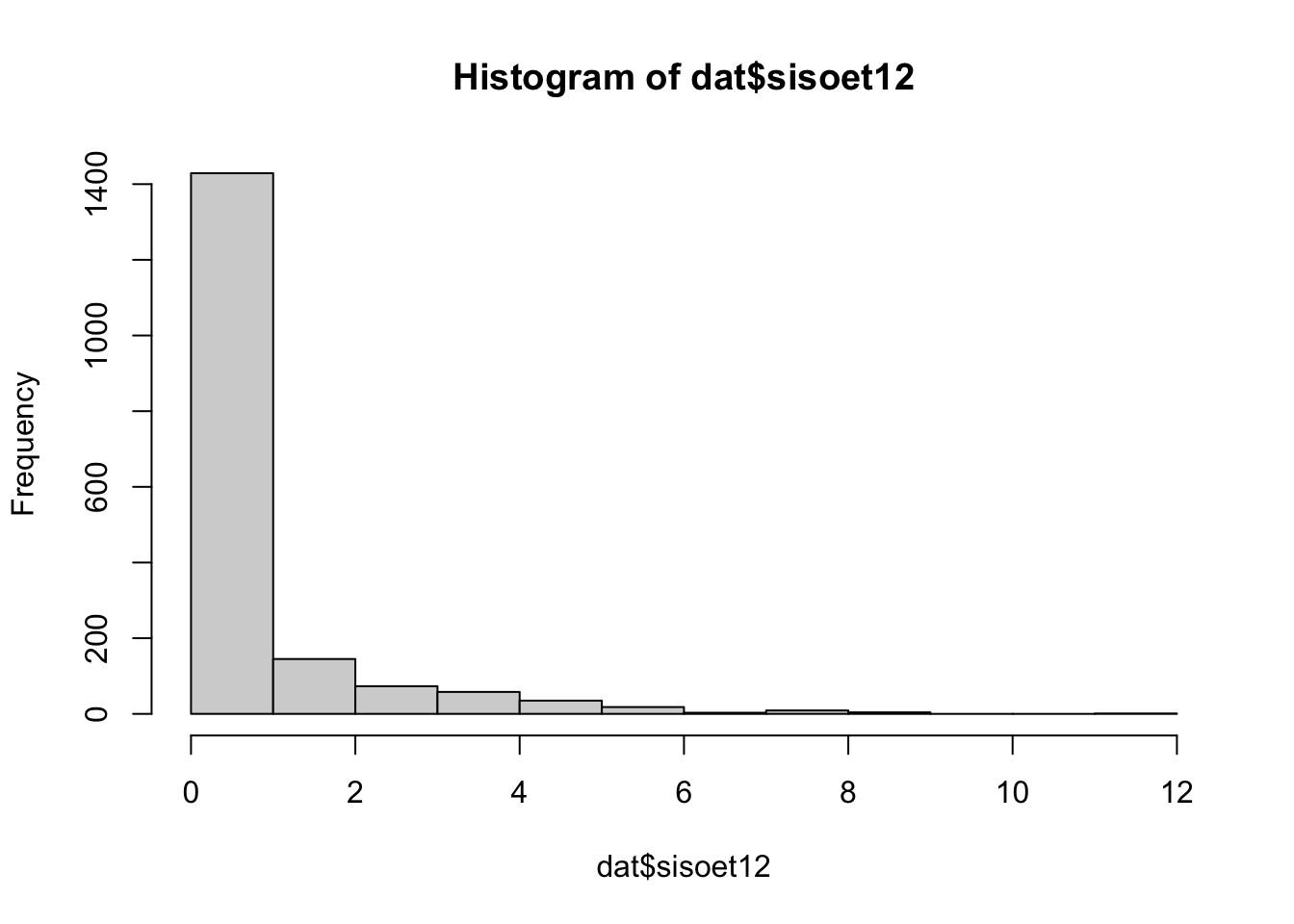
# mother
hist(dat$hyem5)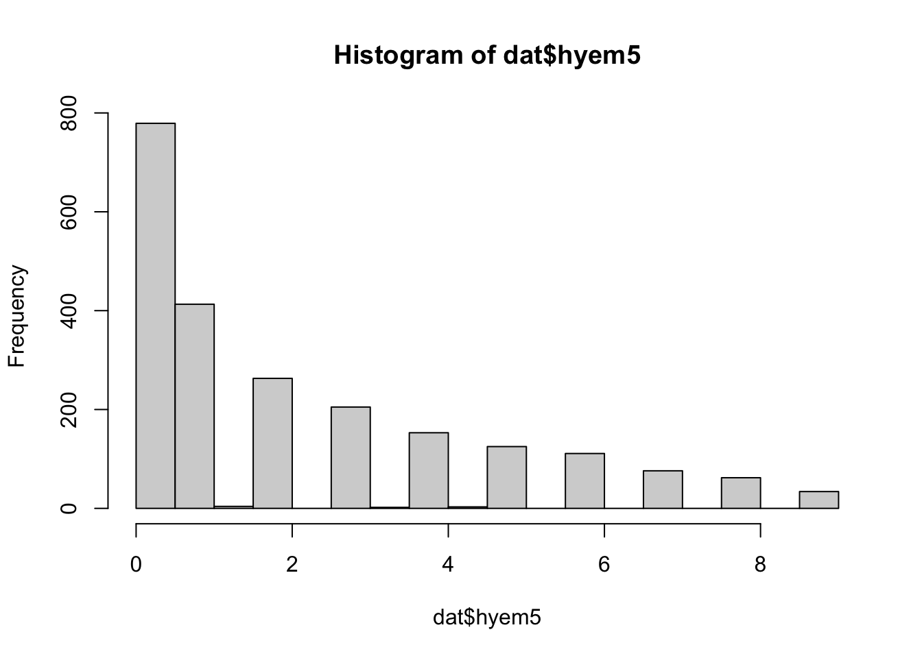
hist(dat$hyem7)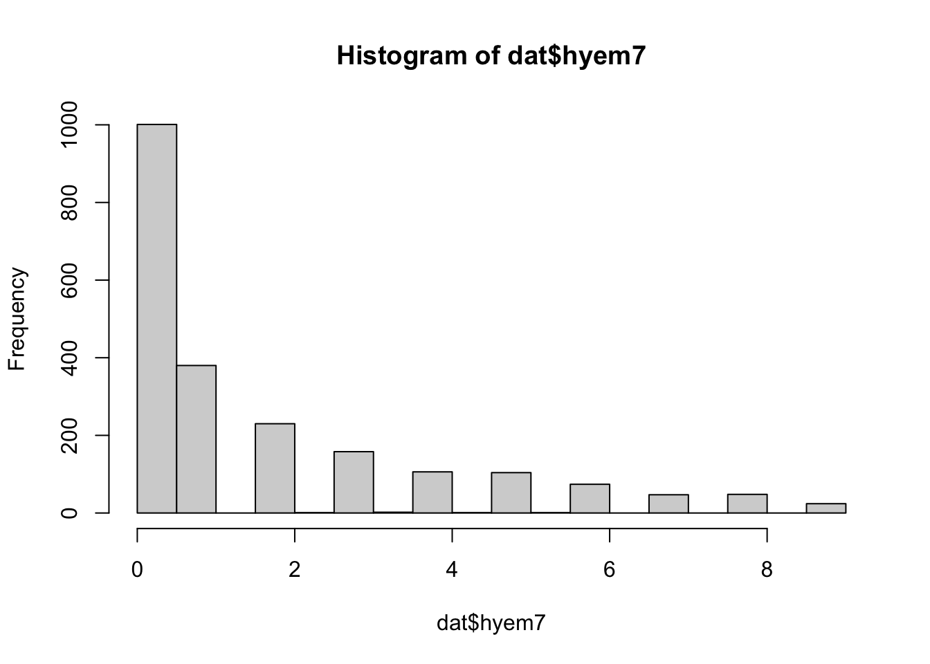
hist(dat$hyem10)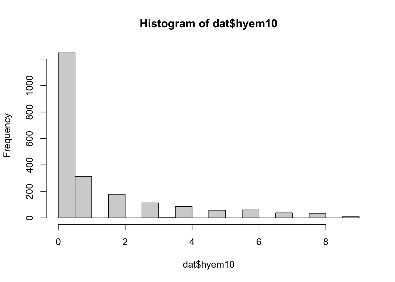
hist(dat$hyem12)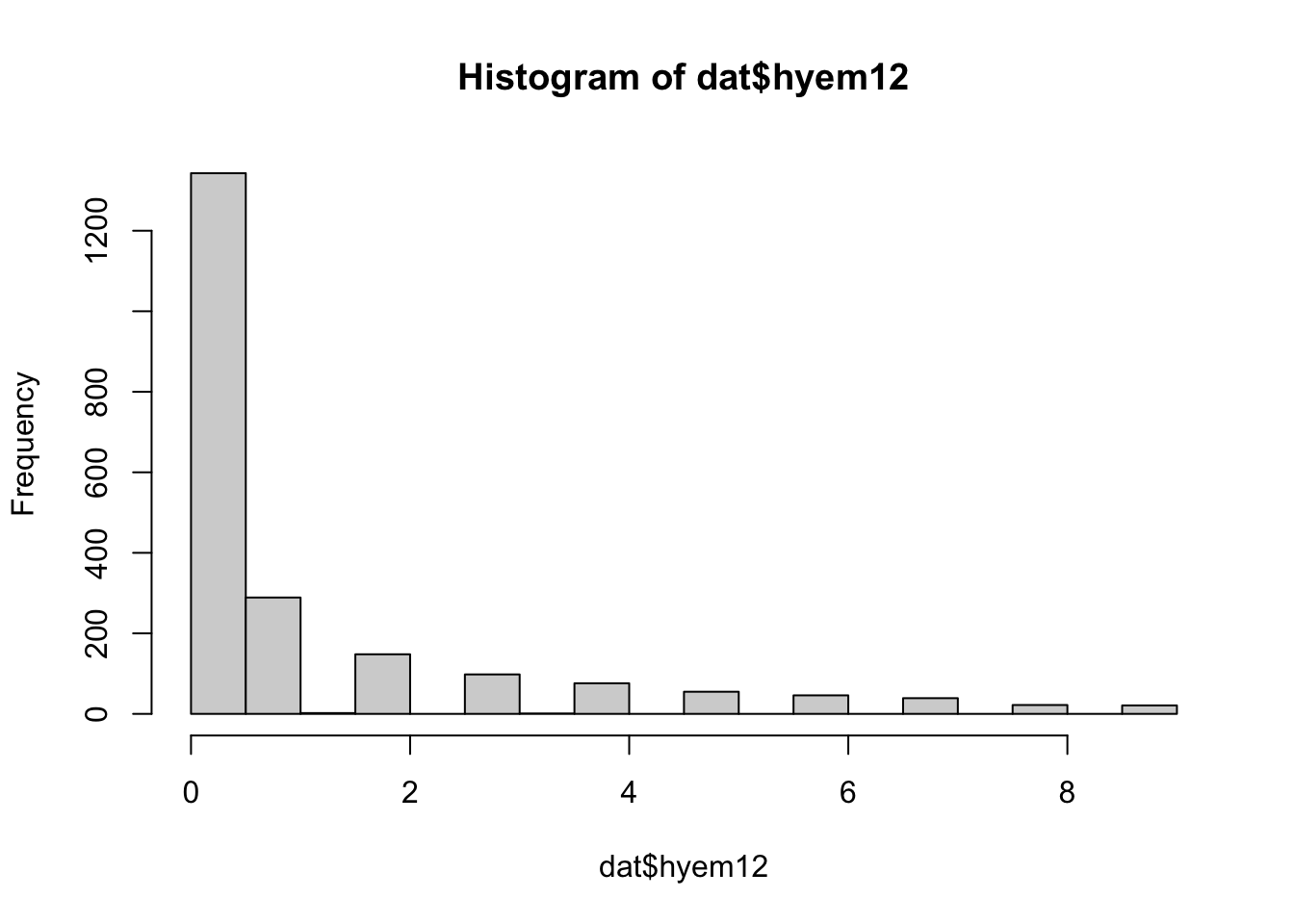
# mother
hist(dat$hyet5)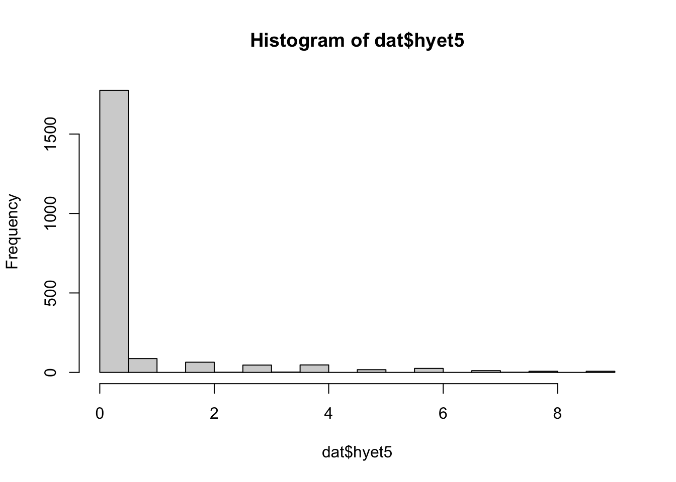
hist(dat$hyet7)
hist(dat$hyet10)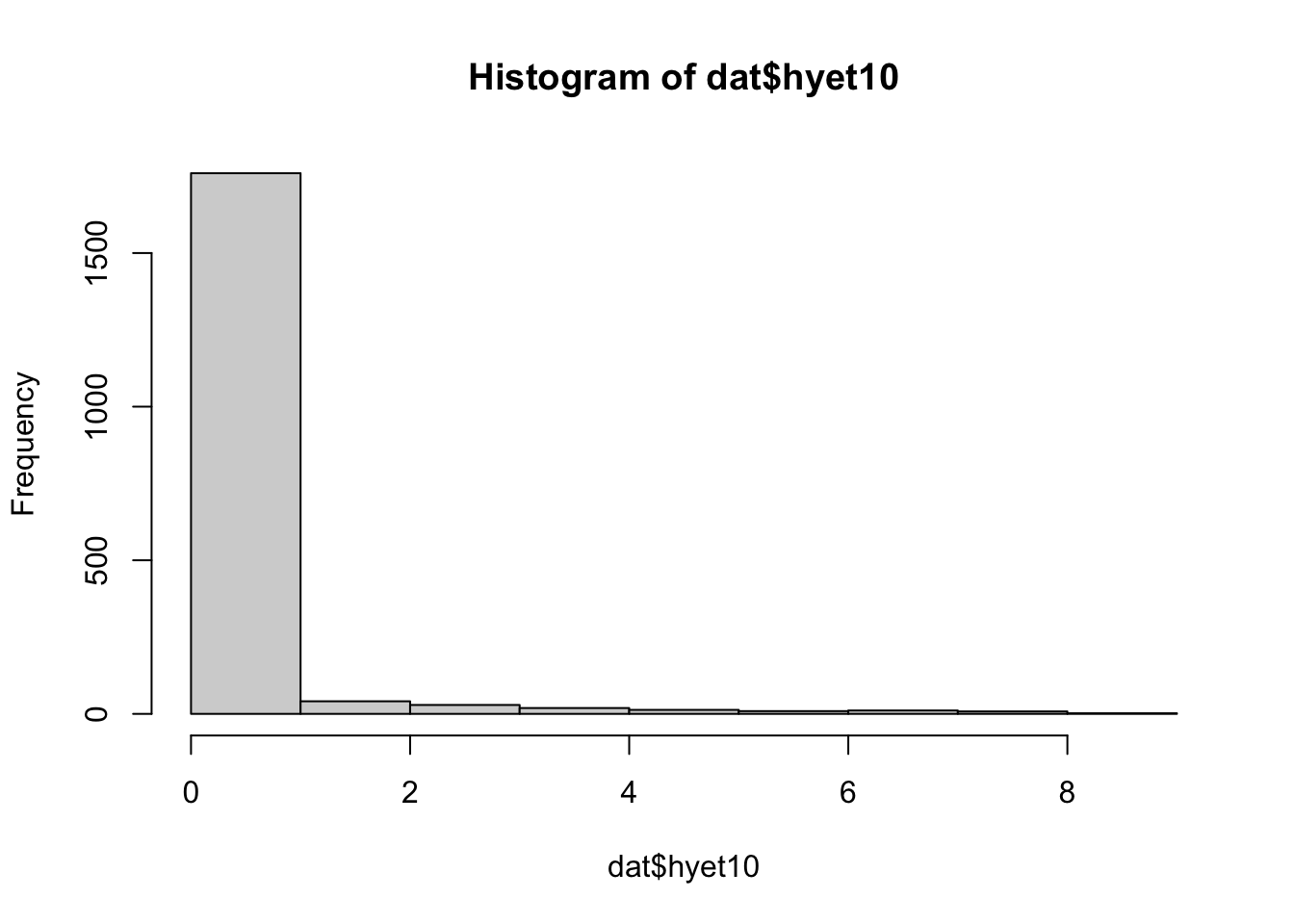
hist(dat$hyet12)
# mother
hist(dat$inem5)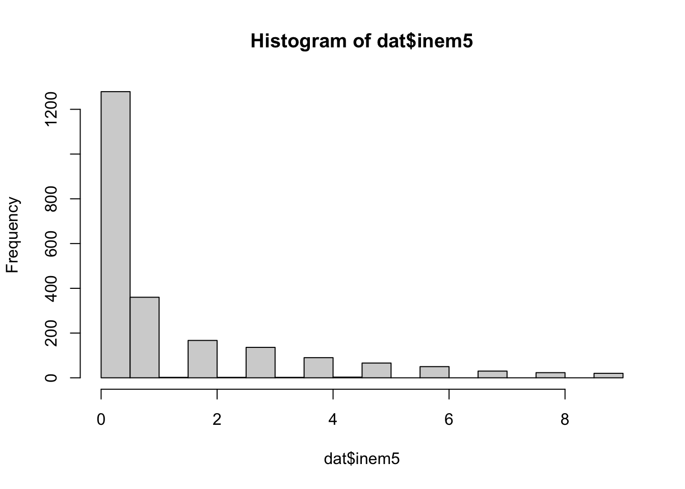
hist(dat$inem7)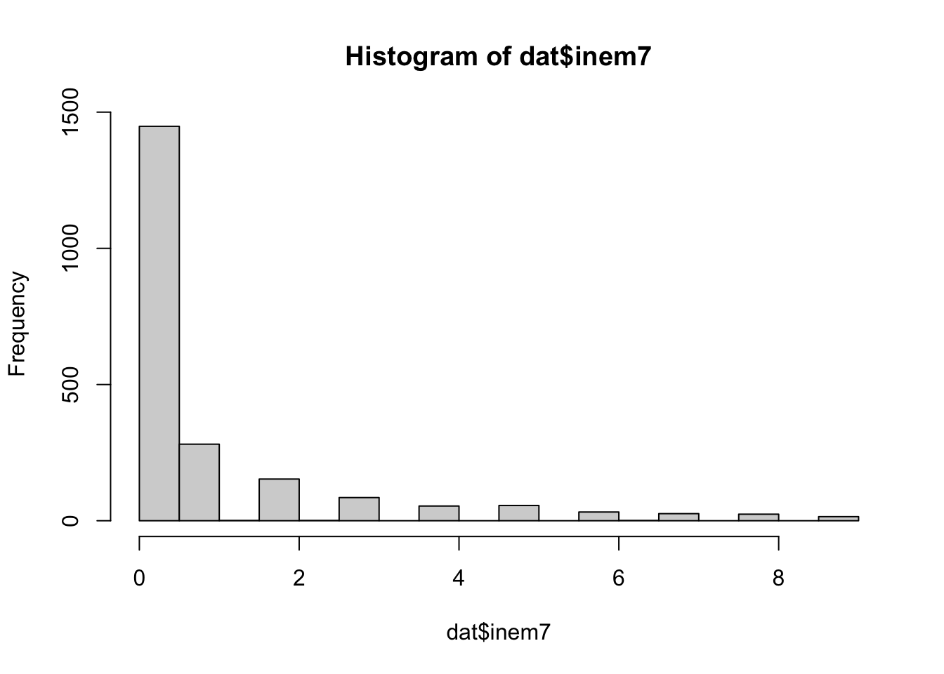
hist(dat$inem10)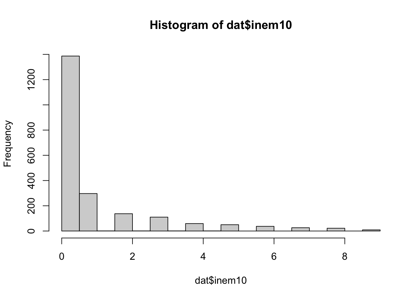
hist(dat$inem12)
# mother
hist(dat$inet5)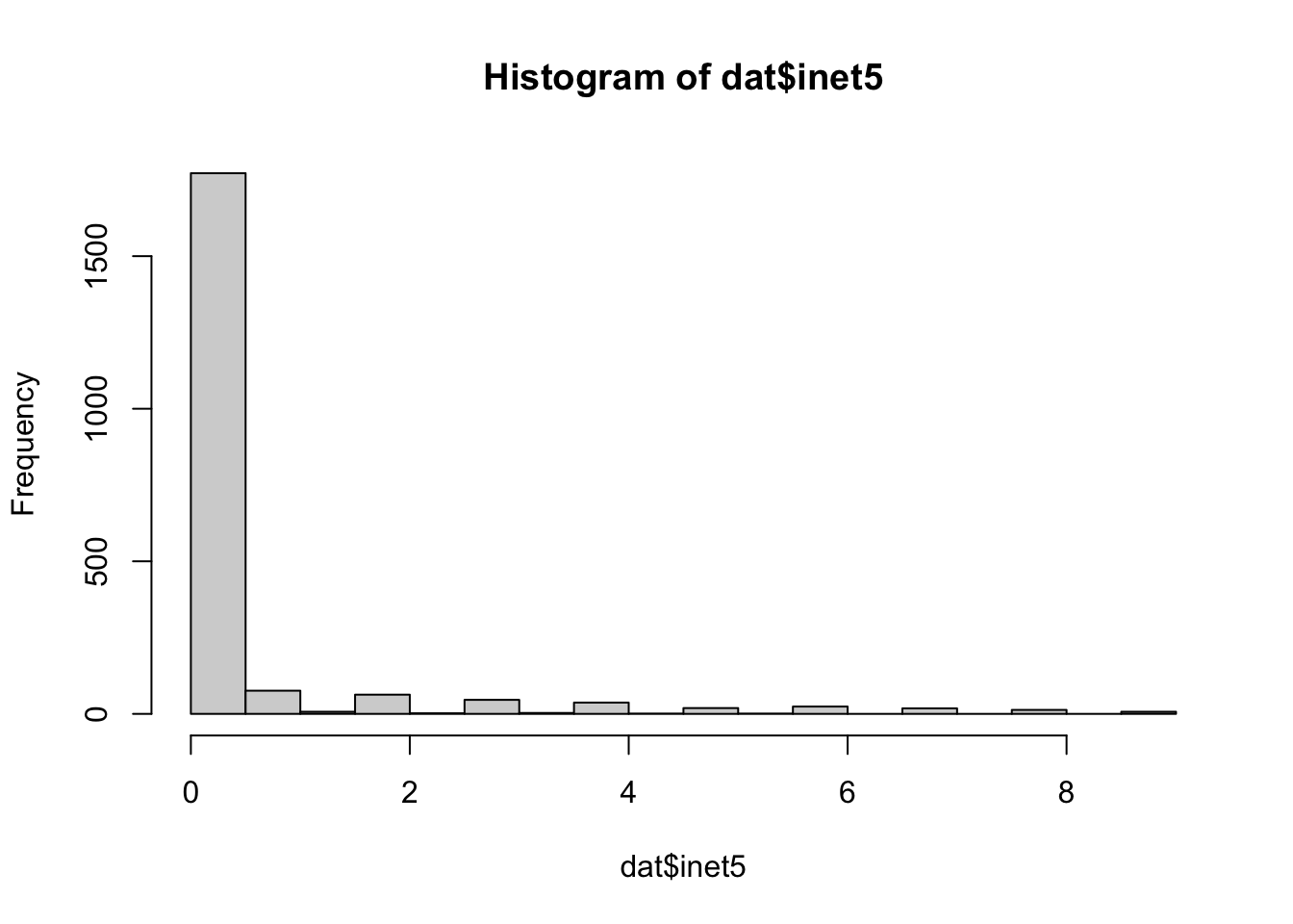
hist(dat$inet7)
hist(dat$inet10)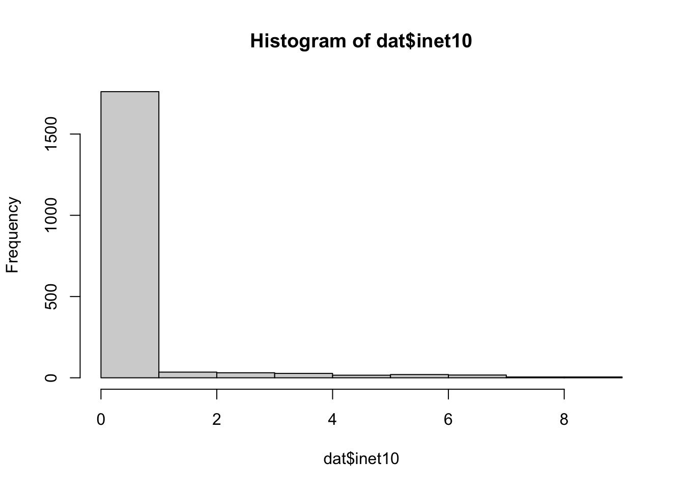
hist(dat$inet12)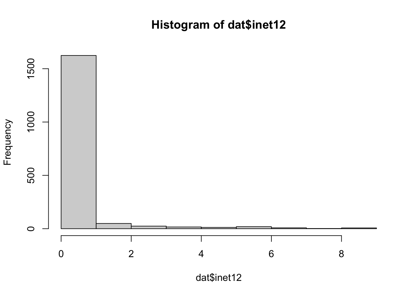
The below introductory notes have been adapted from Hamaker, Kuiper, and Grasman, 2015
The CLPM only accounts for temporal stability through the inclusion of autoregressive parameters. Thus, it is implicitly assumed that every person varies over time around the same means μt and πt, and that there are no trait-like individual differences that endure. this is a rather problematic assumption, as it is difficult to imagine a psychological construct – whether behavioral, cognitive, emotional or psychophysiological – that is not to some extent characterized by stable individual differences (if not for the entire lifespan, then at least for the duration of the study; Hamaker, ). Longitudinal data can actually be thought of as multilevel data, in which occasions are nested within individuals (or other systems, like dyads). When considering this perspective, it becomes clear that we need to separate the within-person level from the between-person level.
The random intercepts cross lagged panel model (RI-CLPM) accounts not only for temporal stability, but also for time-invariant, trait-like stability through the inclusion of a random intercept. The cross-lagged parameters indicate the extent to which the two variables influence each other. The cross-lagged relationships pertain to a process that takes place at the within-person level and they are therefore of key interest when the interest is in reciprocal influences over time within individuals or dyads. The cross-lagged parameter indicates the extent to which the change in y can be predicted from the individual’s prior deviation from their expected score on the other variable, while controlling for the structural change in y and the prior deviation from one’s expected score on y.
The CLPM requires only two waves of data, but the RI-CLPM requires at least three waves of data, in which case there is 1 degree of freedom (df). If the intervals are of the same size, and if we assume that the effects the variables have on each other remain stable over time, we could decide to constrain the lagged parameters over time, giving us an additional 4 df (i.e., 5 df in total). If we are not willing to make these assumptions, and we are not sure whether the effect of the time-invariant stability components κi and ωi are equal over time, we may wish to remove the constraint on the factor loadings. This relaxation may especially be of interest when the observations are made further apart in time, and we expect that we are also measuring some structural changes. However, this would imply that κi and ωi no longer represents random intercepts (as in multilevel modeling), but rather represent latent variables or traits (as common in SEM). Even more so, it would imply we need more waves of data to estimate this model. The gaps in our time waves may be a problem here.
All RI-CLPM models
We conducted RI-CLPM to assess bidirectional associations between social isolation and ADHD symptoms. All models in this script have used sum scores for total ADHD symptoms, hyperactivity symptoms, inattention symptoms, and social isolation. Separate models have been conducted for mother and teacher scores. See the table below for a list of all models and how they are labeled throughout the code.
| Model | Description |
|---|---|
| CLPM | Cross-lagged panel model without random intercepts using mother report and total ADHD scores |
| RICLPM | Basic RI-CLPM model using mother report ratings for AD and SI, and total ADHD scores |
| RICLPM2 | RICLPM but with fixed autoregressive and cross-lagged relations over time |
| RICLPM2a | RICLPM but with fixed ADHD autoregressive over time |
| RICLPM2b | RICLPM but with fixed social isolation autoregressive over time |
| RICLPM2c | RICLPM but with fixed ADHD to social isolation cross-lagged relations over time |
| RICLPM2d | RICLPM but with fixed all cross-lagged relations over time |
| RICLPM3 | RICLPM but with constrained grand means for AD and SI |
| RICLPM_hyp | Basic RI-CLPM model using mother report ratings for AD and SI, and hyperactivity scores |
| RICLPM_hyp2 | RICLPM_hyp but with fixed autoregressive and cross-lagged relations over time |
| RICLPM_hyp2a | RICLPM_hyp but with fixed ADHD autoregressive over time |
| RICLPM_hyp2b | RICLPM_hyp but with fixed social isolation autoregressive over time |
| RICLPM_hyp2c | RICLPM_hyp but with fixed ADHD to social isolation cross-lagged relations over time |
| RICLPM_hyp2d | RICLPM_hyp but with fixed all cross-lagged relations over time |
| RICLPM_hyp3 | RICLPM_hyp but with constrained grand means for AD and SI |
| RICLPM_inat | Basic RI-CLPM model using mother report ratings for AD and SI, and inattention scores |
| RICLPM_inat2 | RICLPM_inat but with fixed autoregressive and cross-lagged relations over time |
| RICLPM_inat2a | RICLPM_inat but with fixed ADHD autoregressive over time |
| RICLPM_inat2b | RICLPM_inat but with fixed social isolation autoregressive over time |
| RICLPM_inat2c | RICLPM_inat but with fixed ADHD to social isolation cross-lagged relations over time |
| RICLPM_inat2d | RICLPM_inat but with fixed all cross-lagged relations over time |
| RICLPM_inat3 | RICLPM_inat but with constrained grand means for AD and SI |
| CLPMt | Cross-lagged panel model without random intercepts using teacher report and total ADHD scores |
| RICLPMt | Basic RI-CLPM model using teacher report ratings for AD and SI, and total ADHD scores |
| RICLPMt2 | RICLPMt but with fixed autoregressive and cross-lagged relations over time |
| RICLPMt3 | RICLPMt but with constrained grand means for AD and SI |
| RICLPMt_hyp | Basic RI-CLPM model using teacher report ratings for AD and SI, and hyperactivity scores |
| RICLPMt_hyp2 | RICLPMt_hyp but with fixed autoregressive and cross-lagged relations over time |
| RICLPMt_hyp3 | RICLPMt_hyp but with constrained grand means for AD and SI |
| RICLPMt_inat | Basic RI-CLPM model using teacher report ratings for AD and SI, and inattention scores |
| RICLPMt_inat2 | RICLPMt_inat but with fixed autoregressive and cross-lagged relations over time |
| RICLPMt_inat3 | RICLPMt_inat but with constrained grand means for AD and SI |
RI-CLPM: Mother report only, total ADHD symptoms
For SEM in lavaan, we use three different formula types: latent variabele definitions (using the =~ operator, which can be read as is “measured by”), regression formulas (using the ~ operator), and (co)variance formulas (using the ~~ operator). The regression formulas are similar to ordinary formulas in R. The expression y1 ~~ y2 allows the residual variances of the two observed variables to be correlated. This is sometimes done if it is believed that the two variables have something in common that is not captured by the latent variables. Note that the two expressions y2 ~~ y4 and y2 ~~ y6, can be combined into the expression y2 ~~ y4 + y6, because the variable on the left of the ~~ operator (y2) is the same. This is just a shorthand notation. In general, to fix a parameter in a lavaan formula, you need to pre-multiply the corresponding variable in the formula by a numerical value. This is called the pre-multiplication mechanism and will be used for many purposes e.g. 1*x2. If you wish to fix the correlation (or covariance) between a pair of latent variables to zero, you need to explicity add a covariance-formula for this pair, and fix the parameter to zero.
To specify the RI-CLPM we need four parts: notes from Mulder’s webpage.
A between part, consisting of the random intercepts. It is specified using the =~ command,
RIx =~ 1*x1 1*x2 ..., where 1* fixes the factor loading to one.A within part, consisting of within-unit fluctuations. It is also specified using the =~ command,
wx1 =~ 1*x1; wx2 =~ 1*x2;The lagged regressions between the within-unit components, using
wx2 ~ wx1 wy1; wx3 ~ wx2 wy2; .... Here, this is written with two variables on the left hand side of the~, this is doing the same thing as calculating just regression paths - but combining DVs that have the same paths leading to them, e.g.wx2 ~ wx1 + wy1andwy2 ~ wx1 + wy1becomeswx2+ wy2 ~ wx1 + wy1.Relevant covariances in both the between and within part. In the within part the components at wave 1, and their residuals at waves 2 and further are correlated within each wave, using
wx1 ~~ wy1; wx2 ~~ wy2;.... We also need to specify their (residual) variances here usingwx1 ~~ wx1; wx2 ~~ wx2; .... For the between part we have to specify the variances and covariance of the random intercepts usingRIx ~~ RIy;.
Tips for interpreting the output: - Model Test User Model: which provides a test statistic, degrees of freedom, and a p-value for the model that was specified by the user. - Model Test Baseline Model: The baseline is a null model, typically in which all of your observed variables are constrained to covary with no other variables (put another way, the covariances are fixed to 0)–just individual variances are estimated.
Cross-lagged panel model (CLPM)
CLPM <- '
  # Estimate the lagged effects between the observed variables.
  tadhdem7 + sisoem7 ~ tadhdem5 + sisoem5
  tadhdem10 + sisoem10 ~ tadhdem7 + sisoem7
  tadhdem12 + sisoem12 ~ tadhdem10 + sisoem10

  # Estimate the covariance between the observed variables at the first wave.
  tadhdem5 ~~ sisoem5 # Covariance

  # Estimate the covariances between the residuals of the observed variables.
  tadhdem7 ~~ sisoem7
  tadhdem10 ~~ sisoem10
  tadhdem12 ~~ sisoem12

  # Estimate the (residual) variance of the observed variables.
  tadhdem5 ~~ tadhdem5 # Variances
  sisoem5 ~~ sisoem5
  tadhdem7 ~~ tadhdem7 # Residual variances
  sisoem7 ~~ sisoem7
  tadhdem10 ~~ tadhdem10
  sisoem10 ~~ sisoem10
  tadhdem12 ~~ tadhdem12
  sisoem12 ~~ sisoem12
'
CLPM.fit <- lavaan(CLPM,
data = dat,
missing = 'ML',
meanstructure = TRUE,
int.ov.free = TRUE,
se = "robust",
estimator = "MLR" #maximum likelihood with robust (Huber-White) standard errors and a scaled (Yuan-Bentler) and robust test statistic
)
CLPM.fit.summary <- summary(CLPM.fit,
fit.measures = TRUE,
standardized = TRUE)lavaan 0.6-10 ended normally after 48 iterations
Estimator ML Optimization method NLMINB Number of model parameters 32
Number of observations 2232 Number of missing patterns 11
Model Test User Model: Standard Robust Test Statistic 459.048 265.187 Degrees of freedom 12 12 P-value (Chi-square) 0.000 0.000 Scaling correction factor 1.731 Yuan-Bentler correction (Mplus variant)
Model Test Baseline Model:
Test statistic 6741.919 3685.347 Degrees of freedom 28 28 P-value 0.000 0.000 Scaling correction factor 1.829
User Model versus Baseline Model:
Comparative Fit Index (CFI) 0.933 0.931 Tucker-Lewis Index (TLI) 0.845 0.838
Robust Comparative Fit Index (CFI) 0.934 Robust Tucker-Lewis Index (TLI) 0.847
Loglikelihood and Information Criteria:
Loglikelihood user model (H0) -36566.211 -36566.211 Scaling correction factor 2.065 for the MLR correction
Loglikelihood unrestricted model (H1) NA NA Scaling correction factor 1.974 for the MLR correction
Akaike (AIC) 73196.422 73196.422 Bayesian (BIC) 73379.163 73379.163 Sample-size adjusted Bayesian (BIC) 73277.494 73277.494
Root Mean Square Error of Approximation:
RMSEA 0.129 0.097 90 Percent confidence interval - lower 0.119 0.090 90 Percent confidence interval - upper 0.139 0.105 P-value RMSEA <= 0.05 0.000 0.000
Robust RMSEA 0.128 90 Percent confidence interval - lower 0.115 90 Percent confidence interval - upper 0.142
Standardized Root Mean Square Residual:
SRMR 0.061 0.061
Parameter Estimates:
Standard errors Sandwich Information bread Observed Observed information based on Hessian
Regressions: Estimate Std.Err z-value P(>|z|) Std.lv Std.all tadhdem7 ~
tadhdem5 0.544 0.023 23.341 0.000 0.544 0.585 sisoem5 0.197 0.058 3.394 0.001 0.197 0.077 sisoem7 ~
tadhdem5 0.042 0.009 4.454 0.000 0.042 0.108 sisoem5 0.526 0.036 14.625 0.000 0.526 0.493 tadhdem10 ~
tadhdem7 0.495 0.027 18.345 0.000 0.495 0.534 sisoem7 0.187 0.061 3.050 0.002 0.187 0.084 sisoem10 ~
tadhdem7 0.053 0.011 4.850 0.000 0.053 0.119 sisoem7 0.503 0.036 14.100 0.000 0.503 0.474 tadhdem12 ~
tadhdem10 0.703 0.026 26.762 0.000 0.703 0.701 sisoem10 0.027 0.045 0.600 0.548 0.027 0.013 sisoem12 ~
tadhdem10 0.060 0.011 5.711 0.000 0.060 0.124 sisoem10 0.581 0.027 21.377 0.000 0.581 0.570
Covariances: Estimate Std.Err z-value P(>|z|) Std.lv Std.all tadhdem5 ~~
sisoem5 1.700 0.177 9.606 0.000 1.700 0.298 .tadhdem7 ~~
.sisoem7 0.692 0.109 6.356 0.000 0.692 0.183 .tadhdem10 ~~
.sisoem10 0.875 0.125 7.026 0.000 0.875 0.224 .tadhdem12 ~~
.sisoem12 0.781 0.127 6.143 0.000 0.781 0.248
Intercepts: Estimate Std.Err z-value P(>|z|) Std.lv Std.all .tadhdem7 0.602 0.076 7.926 0.000 0.602 0.163 .sisoem7 0.335 0.037 9.079 0.000 0.335 0.218 .tadhdem10 0.706 0.070 10.098 0.000 0.706 0.206 .sisoem10 0.462 0.036 12.663 0.000 0.462 0.284 .tadhdem12 0.463 0.060 7.682 0.000 0.463 0.135 .sisoem12 0.278 0.033 8.367 0.000 0.278 0.168 tadhdem5 3.369 0.084 40.091 0.000 3.369 0.849 sisoem5 0.974 0.030 31.967 0.000 0.974 0.677
Variances: Estimate Std.Err z-value P(>|z|) Std.lv Std.all tadhdem5 15.743 0.603 26.122 0.000 15.743 1.000 sisoem5 2.070 0.127 16.358 0.000 2.070 1.000 .tadhdem7 8.510 0.415 20.511 0.000 8.510 0.625 .sisoem7 1.677 0.093 18.038 0.000 1.677 0.713 .tadhdem10 7.971 0.398 20.019 0.000 7.971 0.680 .sisoem10 1.922 0.106 18.100 0.000 1.922 0.726 .tadhdem12 5.907 0.356 16.578 0.000 5.907 0.502 .sisoem12 1.684 0.105 16.006 0.000 1.684 0.612
#Table of model fit
CLPM.fit.summary.fit <- table.model.fit(CLPM.fit.summary)
CLPM.fit.summary.fit
#Table of regression coefficients and covariances (concurrent associations)
CLPM.fit.summary.reg <- table.model.coef(model = CLPM.fit.summary, type = "CLPM", constraints = "No")
CLPM.fit.summary.regThe basic RI-CLPM model (RICLPM)
The code for specifying the basic RI-CLPM is given below.
RICLPM <- '
  # Create between components (random intercepts treated as factors here)
  RIad =~ 1*tadhdem5 + 1*tadhdem7 + 1*tadhdem10 + 1*tadhdem12 #x
  RIsi =~ 1*sisoem5 + 1*sisoem7 + 1*sisoem10 + 1*sisoem12 #y

  # Create within-person centered variables
  wad5 =~ 1*tadhdem5
  wad7 =~ 1*tadhdem7
  wad10 =~ 1*tadhdem10
  wad12 =~ 1*tadhdem12
  wsi5 =~ 1*sisoem5
  wsi7 =~ 1*sisoem7
  wsi10 =~ 1*sisoem10
  wsi12 =~ 1*sisoem12

  # Estimate the lagged effects between the within-person centered variables
  wad7 + wsi7 ~ wad5 + wsi5
  wad10 + wsi10 ~ wad7 + wsi7
  wad12 + wsi12 ~ wad10 + wsi10

  # Estimate the covariance between the within-person centered variables at the first wave
  wad5 ~~ wsi5 # Covariance

  # Estimate the covariances between the residuals of the within-person centered variables (the innovations)
  wad7 ~~ wsi7
  wad10 ~~ wsi10
  wad12 ~~ wsi12

  # Estimate the variance and covariance of the random intercepts
  RIad ~~ RIad
  RIsi ~~ RIsi
  RIad ~~ RIsi

  # Estimate the (residual) variance of the within-person centered variables.
  wad5 ~~ wad5 # Variances
  wsi5 ~~ wsi5
  wad7 ~~ wad7 # Residual variances
  wsi7 ~~ wsi7
  wad10 ~~ wad10
  wsi10 ~~ wsi10
  wad12 ~~ wad12
  wsi12 ~~ wsi12
'
RICLPM.fit <- lavaan(RICLPM, # model
data = dat, # data
missing = 'ML', # how to handle missing data
meanstructure = TRUE, # adds intercepts/means to the model for both observed and latent variables
se = "robust", # robust standard errors
int.ov.free = TRUE, # if FALSE, the intercepts of the observed variables are fixed to zero
estimator = "MLR" #maximum likelihood with robust (Huber-White) standard errors and a scaled (Yuan-Bentler) and robust test statistic
)
RICLPM.fit.summary <- summary(RICLPM.fit,
fit.measures = TRUE,
standardized = TRUE)lavaan 0.6-10 ended normally after 108 iterations
Estimator ML Optimization method NLMINB Number of model parameters 35
Number of observations 2232 Number of missing patterns 11
Model Test User Model: Standard Robust Test Statistic 95.493 61.768 Degrees of freedom 9 9 P-value (Chi-square) 0.000 0.000 Scaling correction factor 1.546 Yuan-Bentler correction (Mplus variant)
Model Test Baseline Model:
Test statistic 6741.919 3685.347 Degrees of freedom 28 28 P-value 0.000 0.000 Scaling correction factor 1.829
User Model versus Baseline Model:
Comparative Fit Index (CFI) 0.987 0.986 Tucker-Lewis Index (TLI) 0.960 0.955
Robust Comparative Fit Index (CFI) 0.988 Robust Tucker-Lewis Index (TLI) 0.962
Loglikelihood and Information Criteria:
Loglikelihood user model (H0) -36384.434 -36384.434 Scaling correction factor 2.084 for the MLR correction
Loglikelihood unrestricted model (H1) NA NA Scaling correction factor 1.974 for the MLR correction
Akaike (AIC) 72838.867 72838.867 Bayesian (BIC) 73038.740 73038.740 Sample-size adjusted Bayesian (BIC) 72927.540 72927.540
Root Mean Square Error of Approximation:
RMSEA 0.066 0.051 90 Percent confidence interval - lower 0.054 0.042 90 Percent confidence interval - upper 0.078 0.061 P-value RMSEA <= 0.05 0.014 0.396
Robust RMSEA 0.064 90 Percent confidence interval - lower 0.049 90 Percent confidence interval - upper 0.079
Standardized Root Mean Square Residual:
SRMR 0.031 0.031
Parameter Estimates:
Standard errors Sandwich Information bread Observed Observed information based on Hessian
Latent Variables: Estimate Std.Err z-value P(>|z|) Std.lv Std.all RIad =~
tadhdem5 1.000 2.568 0.638 tadhdem7 1.000 2.568 0.707 tadhdem10 1.000 2.568 0.750 tadhdem12 1.000 2.568 0.751 RIsi =~
sisoem5 1.000 0.911 0.622 sisoem7 1.000 0.911 0.603 sisoem10 1.000 0.911 0.560 sisoem12 1.000 0.911 0.555 wad5 =~
tadhdem5 1.000 3.098 0.770 wad7 =~
tadhdem7 1.000 2.568 0.707 wad10 =~
tadhdem10 1.000 2.263 0.661 wad12 =~
tadhdem12 1.000 2.258 0.660 wsi5 =~
sisoem5 1.000 1.147 0.783 wsi7 =~
sisoem7 1.000 1.205 0.798 wsi10 =~
sisoem10 1.000 1.347 0.828 wsi12 =~
sisoem12 1.000 1.366 0.832
Regressions: Estimate Std.Err z-value P(>|z|) Std.lv Std.all wad7 ~
wad5 0.233 0.038 6.168 0.000 0.281 0.281 wsi5 0.092 0.087 1.060 0.289 0.041 0.041 wsi7 ~
wad5 0.028 0.015 1.937 0.053 0.073 0.073 wsi5 0.236 0.060 3.917 0.000 0.224 0.224 wad10 ~
wad7 0.022 0.064 0.343 0.731 0.025 0.025 wsi7 0.171 0.115 1.487 0.137 0.091 0.091 wsi10 ~
wad7 0.035 0.023 1.486 0.137 0.066 0.066 wsi7 0.266 0.061 4.333 0.000 0.238 0.238 wad12 ~
wad10 0.314 0.066 4.773 0.000 0.315 0.315 wsi10 0.041 0.074 0.557 0.577 0.025 0.025 wsi12 ~
wad10 0.026 0.029 0.897 0.370 0.044 0.044 wsi10 0.424 0.043 9.977 0.000 0.418 0.418
Covariances: Estimate Std.Err z-value P(>|z|) Std.lv Std.all wad5 ~~
wsi5 0.748 0.156 4.782 0.000 0.210 0.210 .wad7 ~~
.wsi7 0.441 0.129 3.424 0.001 0.154 0.154 .wad10 ~~
.wsi10 0.752 0.158 4.764 0.000 0.257 0.257 .wad12 ~~
.wsi12 0.592 0.111 5.308 0.000 0.225 0.225 RIad ~~
RIsi 1.095 0.142 7.697 0.000 0.468 0.468
Intercepts: Estimate Std.Err z-value P(>|z|) Std.lv Std.all .tadhdem5 3.369 0.084 40.093 0.000 3.369 0.837 .tadhdem7 2.627 0.079 33.386 0.000 2.627 0.723 .tadhdem10 2.192 0.073 29.924 0.000 2.192 0.640 .tadhdem12 2.033 0.073 27.728 0.000 2.033 0.595 .sisoem5 0.974 0.030 31.967 0.000 0.974 0.665 .sisoem7 0.987 0.033 30.133 0.000 0.987 0.654 .sisoem10 1.097 0.035 31.447 0.000 1.097 0.675 .sisoem12 1.048 0.036 29.455 0.000 1.048 0.638 RIad 0.000 0.000 0.000 RIsi 0.000 0.000 0.000 wad5 0.000 0.000 0.000 .wad7 0.000 0.000 0.000 .wad10 0.000 0.000 0.000 .wad12 0.000 0.000 0.000 wsi5 0.000 0.000 0.000 .wsi7 0.000 0.000 0.000 .wsi10 0.000 0.000 0.000 .wsi12 0.000 0.000 0.000
Variances: Estimate Std.Err z-value P(>|z|) Std.lv Std.all RIad 6.596 0.487 13.536 0.000 1.000 1.000 RIsi 0.829 0.101 8.174 0.000 1.000 1.000 wad5 9.596 0.509 18.871 0.000 1.000 1.000 wsi5 1.316 0.126 10.462 0.000 1.000 1.000 .wad7 6.027 0.421 14.299 0.000 0.914 0.914 .wsi7 1.361 0.102 13.392 0.000 0.937 0.937 .wad10 5.070 0.526 9.639 0.000 0.990 0.990 .wsi10 1.692 0.113 14.914 0.000 0.933 0.933 .wad12 4.568 0.305 14.958 0.000 0.896 0.896 .wsi12 1.518 0.097 15.628 0.000 0.813 0.813 .tadhdem5 0.000 0.000 0.000 .tadhdem7 0.000 0.000 0.000 .tadhdem10 0.000 0.000 0.000 .tadhdem12 0.000 0.000 0.000 .sisoem5 0.000 0.000 0.000 .sisoem7 0.000 0.000 0.000 .sisoem10 0.000 0.000 0.000 .sisoem12 0.000 0.000 0.000
#Table of model fit
RICLPM.fit.summary.fit <- table.model.fit(RICLPM.fit.summary)
#Table of regression coefficients and covariances (concurrent associations)
RICLPM.fit.summary.reg <- table.model.coef(model = RICLPM.fit.summary, type = "RICLPM", constraints = "No")
Comparison between CLPM and RI-CLPM
The use of the chi-square difference test is wide-spread in the SEM community to test constraints on parameters. However, when constraints are placed on the bound of the parameter space, we should use the chi-bar-square test (χ¯2-test) (Stoel et al. 2006). For example, if we constrain the variances of all random intercepts (and their covariance) in the RI-CLPM to zero, we obtain a model that is nested under the RI-CLPM, and that is statistically equivalent to the traditional cross-lagged panel model (CLPM). Below you can find R code for performing the chi-bar-square test (code by Rebecca M. Kuiper) for comparing these two models. It involves
- fitting both the RI-CLPM (RICLPM.fit) and CLPM (CLPM.fit); (already done - this is the non-constrained RI-CLPM - RICLPM.fit)
- extracting the covariance matrix of the random intercepts;
- extracting the χ2 and degrees of freedom of both models; and
- performing the χ¯2-test using the ChiBarSq.DiffTest package (Kuiper 2020).
# # Step 2: check which indices you need to get the covariance matrix of the random intercepts.
# vcov(RICLPM.fit) # Full covariance matrix
# indices <- c(17, 18) # From the matrix above, you need the variance of each intercept. Here, the 17th and the 18th indices regard the random intercepts.
# number <- length(indices) # Number of random intercepts
# cov.matrix <- vcov(RICLPM.fit)[indices, indices] # Extract full covariance matrix of the random intercepts
#
# # Step 3: call Chi square and degrees of freedom from each model
# Chi2_CLPM <- summary(CLPM.fit, fit.measures = TRUE)[1]$FIT[c("chisq")] # Extract chi-square value of CLPM
# Chi2_RICLPM <- summary(RICLPM.fit, fit.measures = TRUE)[1]$FIT[c("chisq")] # Extract chi-square value of RI-CLPM
#
# df_CLPM <- summary(CLPM.fit, fit.measures = TRUE)[1]$FIT[c("df")] # Extract df of CLPM
# df_RICLPM <- summary(RICLPM.fit, fit.measures = TRUE)[1]$FIT[c("df")] # Extract df of RI-CLPM
#
# # Step 4: run function to do chi-bar-square test (and also obtain Chi-bar-square weigths)
# ChiBar2DiffTest <- ChiBarSq.DiffTest(number, cov.matrix, Chi2_CLPM, Chi2_RICLPM, df_CLPM, df_RICLPM)
# ChiBar2DiffTest
# ChiBar2DiffTest$p_value
RI-CLPM Constraints over time
Imposing constraints to the model can be achieved through pre-multiplication. It means that we have to prepend the number that we want to fix the parameter to, and an asterisk, to the parameter in the model specification. For example, F =~ 0*x1 fixes the factor loading of item x1 to factor F to 0. Using pre-multiplication we can also constrain parameters to be the same by giving them the same label. Below we specify an RI-CLPM with the following constraints:
- fixed auto-regressive and cross-lagged relations over time,
wx2 ~ a*wx1 + b*wy1; ... - time-invariant (residual) (co-)variances in the within-person part
wx2 ~~ cov*wy2; ...,wx2 ~~ vx*wx2; ..., andwy2 ~~ vy*wy2; ... - constrained grand means over time,
x1 + ... ~ mx*1andy1 + ... ~ my*1
Fixed autoregressive and cross-lagged relations over time (RICLPM2)
a = lag in ad b = lag in si c = cross lag ad->si d = cross lag si->ad
From Mulder and Hamaker (2021): We may consider testing if the lagged regression coefficients are time-invariant. This can be done by comparing the fit of a model with constrained regression coefficients (over time), with the fit of a model where these parameters are freely estimated (i.e., the unconstrained model). If this chi-square difference test is non-significant, this implies the constraints are tenable and the dynamics of the process are time-invariant. If the constraints are not tenable, this could be indicative of some kind of developmental process taking place during the time span covered by the study. In this context, it is important to realize that the lagged regression coefficients depend critically on the time interval between the repeated measures. Hence, constraining the lagged parameters to be invariant across consecutive waves only makes sense when the time interval between the occasions is (approximately) equal.
Constraining all lag and crosslag parameters at once (RICLPM2)
RICLPM2 <- '
  # Create between components (random intercepts treated as factors here)
  RIad =~ 1*tadhdem5 + 1*tadhdem7 + 1*tadhdem10 + 1*tadhdem12 #x
  RIsi =~ 1*sisoem5 + 1*sisoem7 + 1*sisoem10 + 1*sisoem12 #y

  # Create within-person centered variables
  wad5 =~ 1*tadhdem5
  wad7 =~ 1*tadhdem7
  wad10 =~ 1*tadhdem10
  wad12 =~ 1*tadhdem12
  wsi5 =~ 1*sisoem5
  wsi7 =~ 1*sisoem7
  wsi10 =~ 1*sisoem10
  wsi12 =~ 1*sisoem12


  # Constrained lagged effects between the within-person centered variables.
  wad7 ~ a*wad5 + d*wsi5
  wsi7 ~ c*wad5 + b*wsi5

  wad10 ~ a*wad7 + d*wsi7
  wsi10 ~ c*wad7 + b*wsi7

  wad12 ~ a*wad10 + d*wsi10
  wsi12 ~ c*wad10 + b*wsi10

  # Estimate the covariance between the within-person centered variables at the first wave
  wad5 ~~ wsi5 # Covariance

  # Estimate the covariances between the residuals of the within-person centered variables (the innovations)
  wad7 ~~ wsi7
  wad10 ~~ wsi10
  wad12 ~~ wsi12

  # Estimate the variance and covariance of the random intercepts
  RIad ~~ RIad
  RIsi ~~ RIsi
  RIad ~~ RIsi

  # Estimate the (residual) variance of the within-person centered variables.
  wad5 ~~ wad5 # Variances
  wsi5 ~~ wsi5
  wad7 ~~ wad7 # Residual variances
  wsi7 ~~ wsi7
  wad10 ~~ wad10
  wsi10 ~~ wsi10
  wad12 ~~ wad12
  wsi12 ~~ wsi12
'
RICLPM2.fit <- lavaan(RICLPM2,
data = dat,
missing = 'ML',
meanstructure = TRUE,
int.ov.free = TRUE,
se = "robust",
estimator = "MLR" #maximum likelihood with robust (Huber-White) standard errors and a scaled (Yuan-Bentler) and robust test statistic
) lavTestLRT(RICLPM.fit, RICLPM2.fit, method = "satorra.bentler.2010")RICLPM2 is significantly worse fit compared to RICLPM according to the Chi square test.
Constraining lag in ADHD parameter (RICLPM2a)
Now we will test the constraints based on the following steps recommended by Curran and Bauer: 1. Estimate the baseline model where all parameters are freely estimated (The basic RI-CLPM) 2. Impose equlaity constraints on one set of stabilities (within variable lags). Use LRT tests to see if he fit becomes significantly worse. 3. Impose equality constraints on the next set of stabilities. Compare this to wither model 1 (baseline/basic) if step 2 was significant. Compare to model 2 if step 2 was non-significant. Non-sig LRT = not significantly worse fit 4. Repeat for first set of cross-lags 5. Repeat for second set of cross-lags
RICLPM2a <- '
  # Create between components (random intercepts treated as factors here)
  RIad =~ 1*tadhdem5 + 1*tadhdem7 + 1*tadhdem10 + 1*tadhdem12 #x
  RIsi =~ 1*sisoem5 + 1*sisoem7 + 1*sisoem10 + 1*sisoem12 #y

  # Create within-person centered variables
  wad5 =~ 1*tadhdem5
  wad7 =~ 1*tadhdem7
  wad10 =~ 1*tadhdem10
  wad12 =~ 1*tadhdem12
  wsi5 =~ 1*sisoem5
  wsi7 =~ 1*sisoem7
  wsi10 =~ 1*sisoem10
  wsi12 =~ 1*sisoem12


  # Constrained lagged effects between the within-person centered variables.
  wad7 ~ a*wad5 + wsi5
  wsi7 ~ wad5 + wsi5

  wad10 ~ a*wad7 + wsi7
  wsi10 ~ wad7 + wsi7

  wad12 ~ a*wad10 + wsi10
  wsi12 ~ wad10 + wsi10

  # Estimate the covariance between the within-person centered variables at the first wave
  wad5 ~~ wsi5 # Covariance

  # Estimate the covariances between the residuals of the within-person centered variables (the innovations)
  wad7 ~~ wsi7
  wad10 ~~ wsi10
  wad12 ~~ wsi12

  # Estimate the variance and covariance of the random intercepts
  RIad ~~ RIad
  RIsi ~~ RIsi
  RIad ~~ RIsi

  # Estimate the (residual) variance of the within-person centered variables.
  wad5 ~~ wad5 # Variances
  wsi5 ~~ wsi5
  wad7 ~~ wad7 # Residual variances
  wsi7 ~~ wsi7
  wad10 ~~ wad10
  wsi10 ~~ wsi10
  wad12 ~~ wad12
  wsi12 ~~ wsi12
'
RICLPM2a.fit <- lavaan(RICLPM2a,
data = dat,
missing = 'ML',
meanstructure = TRUE,
int.ov.free = TRUE,
se = "robust",
estimator = "MLR" #maximum likelihood with robust (Huber-White) standard errors and a scaled (Yuan-Bentler) and robust test statistic
) lavTestLRT(RICLPM.fit, RICLPM2a.fit, method = "satorra.bentler.2010")RICLPM2a is significantly worse fit compared to RICLPM. Now we will constrain the other set of stability coefficients: lag in si (b)
Constrained grand means (RICLPM3)
The grand means are the means over all units per occasion. These grand means may be time-varying, or may be fixed to be invariant over time.
RICLPM3 <- '
  # Create between components (random intercepts treated as factors here)
  RIad =~ 1*tadhdem5 + 1*tadhdem7 + 1*tadhdem10 + 1*tadhdem12 #x
  RIsi =~ 1*sisoem5 + 1*sisoem7 + 1*sisoem10 + 1*sisoem12 #y

  # Create within-person centered variables
  wad5 =~ 1*tadhdem5
  wad7 =~ 1*tadhdem7
  wad10 =~ 1*tadhdem10
  wad12 =~ 1*tadhdem12
  wsi5 =~ 1*sisoem5
  wsi7 =~ 1*sisoem7
  wsi10 =~ 1*sisoem10
  wsi12 =~ 1*sisoem12

  # Constrained lagged effects between the within-person centered variables.
  wad7 ~ wad5 + wsi5
  wsi7 ~ wad5 + wsi5
  wad10 ~ wad7 + wsi7
  wsi10 ~ wad7 + wsi7
  wad12 ~ wad10 + wsi10
  wsi12 ~ wad10 + wsi10

  # Estimate the covariance between the within-person centered variables at the first wave
  wad5 ~~ wsi5 # Covariance

  # Estimate the covariances between the residuals of the within-person centered variables (the innovations)
  wad7 ~~ wsi7
  wad10 ~~ wsi10
  wad12 ~~ wsi12

  # Estimate the variance and covariance of the random intercepts
  RIad ~~ RIad
  RIsi ~~ RIsi
  RIad ~~ RIsi

  # Estimate the (residual) variance of the within-person centered variables
  wad5 ~~ wad5 # Variances
  wsi5 ~~ wsi5
  wad7 ~~ wad7 # Residual variances
  wsi7 ~~ wsi7
  wad10 ~~ wad10
  wsi10 ~~ wsi10
  wad12 ~~ wad12
  wsi12 ~~ wsi12

  # Constrain the grand means over time
  tadhdem5 + tadhdem7 + tadhdem10 + tadhdem12 ~ mad*1
  sisoem5 + sisoem7 + sisoem10 + sisoem12 ~ msi*1
'
RICLPM3.fit <- lavaan(RICLPM3,
data = dat,
missing = 'ML',
meanstructure = TRUE,
int.ov.free = TRUE,
se = "robust",
estimator = "MLR" #maximum likelihood with robust (Huber-White) standard errors and a scaled (Yuan-Bentler) and robust test statistic
) lavTestLRT(RICLPM.fit, RICLPM3.fit, method = "satorra.bentler.2010") If the grand means cannot be constrained to be invariant over time, this implies that on average there is some change in this variable over time, which may reflect some occasion-specific effect, or a developmental trend. By allowing the means to freely vary over time, we account for such average changes over time.
This makes sense as we have shown variation in social isolation over time and other literature has shown variation in ADHD over time.
RI-CLPM: Mother report only, Hyperactive/Impulsive ADHD symptoms
The basic RI-CLPM model (RICLPM_hyp)
The code for specifying the basic RI-CLPM is given below.
RICLPM_hyp <- '
  # Create between components (random intercepts treated as factors here)
  RIad =~ 1*hyem5 + 1*hyem7 + 1*hyem10 + 1*hyem12 #x
  RIsi =~ 1*sisoem5 + 1*sisoem7 + 1*sisoem10 + 1*sisoem12 #y

  # Create within-person centered variables
  wad5 =~ 1*hyem5
  wad7 =~ 1*hyem7
  wad10 =~ 1*hyem10
  wad12 =~ 1*hyem12
  wsi5 =~ 1*sisoem5
  wsi7 =~ 1*sisoem7
  wsi10 =~ 1*sisoem10
  wsi12 =~ 1*sisoem12

  # Estimate the lagged effects between the within-person centered variables
  wad7 + wsi7 ~ wad5 + wsi5
  wad10 + wsi10 ~ wad7 + wsi7
  wad12 + wsi12 ~ wad10 + wsi10

  # Estimate the covariance between the within-person centered variables at the first wave
  wad5 ~~ wsi5 # Covariance

  # Estimate the covariances between the residuals of the within-person centered variables (the innovations)
  wad7 ~~ wsi7
  wad10 ~~ wsi10
  wad12 ~~ wsi12

  # Estimate the variance and covariance of the random intercepts
  RIad ~~ RIad
  RIsi ~~ RIsi
  RIad ~~ RIsi

  # Estimate the (residual) variance of the within-person centered variables.
  wad5 ~~ wad5 # Variances
  wsi5 ~~ wsi5
  wad7 ~~ wad7 # Residual variances
  wsi7 ~~ wsi7
  wad10 ~~ wad10
  wsi10 ~~ wsi10
  wad12 ~~ wad12
  wsi12 ~~ wsi12
'
RICLPM_hyp.fit <- lavaan(RICLPM_hyp, # model
data = dat, # data
missing = 'ML', # how to handle missing data
meanstructure = TRUE, # adds intercepts/means to the model for both observed and latent variables
se = "robust", # robust standard errors
int.ov.free = TRUE, # if FALSE, the intercepts of the observed variables are fixed to zero
estimator = "MLR" #maximum likelihood with robust (Huber-White) standard errors and a scaled (Yuan-Bentler) and robust test statistic
)
RICLPM_hyp.fit.summary <- summary(RICLPM_hyp.fit,
fit.measures = TRUE,
standardized = TRUE)lavaan 0.6-10 ended normally after 80 iterations
Estimator ML Optimization method NLMINB Number of model parameters 35
Number of observations 2232 Number of missing patterns 11
Model Test User Model: Standard Robust Test Statistic 76.720 51.533 Degrees of freedom 9 9 P-value (Chi-square) 0.000 0.000 Scaling correction factor 1.489 Yuan-Bentler correction (Mplus variant)
Model Test Baseline Model:
Test statistic 6316.653 3679.908 Degrees of freedom 28 28 P-value 0.000 0.000 Scaling correction factor 1.717
User Model versus Baseline Model:
Comparative Fit Index (CFI) 0.989 0.988 Tucker-Lewis Index (TLI) 0.966 0.964
Robust Comparative Fit Index (CFI) 0.990 Robust Tucker-Lewis Index (TLI) 0.969
Loglikelihood and Information Criteria:
Loglikelihood user model (H0) -32076.243 -32076.243 Scaling correction factor 1.939 for the MLR correction
Loglikelihood unrestricted model (H1) NA NA Scaling correction factor 1.847 for the MLR correction
Akaike (AIC) 64222.485 64222.485 Bayesian (BIC) 64422.358 64422.358 Sample-size adjusted Bayesian (BIC) 64311.157 64311.157
Root Mean Square Error of Approximation:
RMSEA 0.058 0.046 90 Percent confidence interval - lower 0.046 0.036 90 Percent confidence interval - upper 0.070 0.056 P-value RMSEA <= 0.05 0.122 0.726
Robust RMSEA 0.056 90 Percent confidence interval - lower 0.042 90 Percent confidence interval - upper 0.071
Standardized Root Mean Square Residual:
SRMR 0.027 0.027
Parameter Estimates:
Standard errors Sandwich Information bread Observed Observed information based on Hessian
Latent Variables: Estimate Std.Err z-value P(>|z|) Std.lv Std.all RIad =~
hyem5 1.000 1.484 0.610 hyem7 1.000 1.484 0.669 hyem10 1.000 1.484 0.741 hyem12 1.000 1.484 0.752 RIsi =~
sisoem5 1.000 0.918 0.628 sisoem7 1.000 0.918 0.609 sisoem10 1.000 0.918 0.564 sisoem12 1.000 0.918 0.557 wad5 =~
hyem5 1.000 1.927 0.792 wad7 =~
hyem7 1.000 1.648 0.743 wad10 =~
hyem10 1.000 1.343 0.671 wad12 =~
hyem12 1.000 1.301 0.659 wsi5 =~
sisoem5 1.000 1.139 0.779 wsi7 =~
sisoem7 1.000 1.197 0.793 wsi10 =~
sisoem10 1.000 1.343 0.826 wsi12 =~
sisoem12 1.000 1.369 0.831
Regressions: Estimate Std.Err z-value P(>|z|) Std.lv Std.all wad7 ~
wad5 0.269 0.032 8.457 0.000 0.315 0.315 wsi5 0.046 0.052 0.883 0.377 0.032 0.032 wsi7 ~
wad5 0.040 0.022 1.830 0.067 0.064 0.064 wsi5 0.231 0.060 3.846 0.000 0.220 0.220 wad10 ~
wad7 0.067 0.049 1.360 0.174 0.082 0.082 wsi7 0.100 0.064 1.577 0.115 0.089 0.089 wsi10 ~
wad7 0.040 0.032 1.271 0.204 0.049 0.049 wsi7 0.266 0.063 4.226 0.000 0.237 0.237 wad12 ~
wad10 0.256 0.062 4.155 0.000 0.264 0.264 wsi10 0.020 0.043 0.461 0.645 0.020 0.020 wsi12 ~
wad10 0.054 0.045 1.200 0.230 0.053 0.053 wsi10 0.424 0.042 9.987 0.000 0.416 0.416
Covariances: Estimate Std.Err z-value P(>|z|) Std.lv Std.all wad5 ~~
wsi5 0.312 0.087 3.608 0.000 0.142 0.142 .wad7 ~~
.wsi7 0.208 0.070 2.956 0.003 0.115 0.115 .wad10 ~~
.wsi10 0.414 0.091 4.539 0.000 0.239 0.239 .wad12 ~~
.wsi12 0.299 0.066 4.548 0.000 0.194 0.194 RIad ~~
RIsi 0.564 0.078 7.245 0.000 0.414 0.414
Intercepts: Estimate Std.Err z-value P(>|z|) Std.lv Std.all .hyem5 2.160 0.051 42.248 0.000 2.160 0.888 .hyem7 1.682 0.048 35.127 0.000 1.682 0.758 .hyem10 1.227 0.043 28.619 0.000 1.227 0.613 .hyem12 1.105 0.042 26.128 0.000 1.105 0.560 .sisoem5 0.974 0.030 31.968 0.000 0.974 0.666 .sisoem7 0.987 0.033 30.130 0.000 0.987 0.655 .sisoem10 1.097 0.035 31.447 0.000 1.097 0.674 .sisoem12 1.049 0.036 29.466 0.000 1.049 0.636 RIad 0.000 0.000 0.000 RIsi 0.000 0.000 0.000 wad5 0.000 0.000 0.000 .wad7 0.000 0.000 0.000 .wad10 0.000 0.000 0.000 .wad12 0.000 0.000 0.000 wsi5 0.000 0.000 0.000 .wsi7 0.000 0.000 0.000 .wsi10 0.000 0.000 0.000 .wsi12 0.000 0.000 0.000
Variances: Estimate Std.Err z-value P(>|z|) Std.lv Std.all RIad 2.202 0.145 15.160 0.000 1.000 1.000 RIsi 0.843 0.102 8.298 0.000 1.000 1.000 wad5 3.713 0.168 22.070 0.000 1.000 1.000 wsi5 1.297 0.124 10.475 0.000 1.000 1.000 .wad7 2.435 0.136 17.949 0.000 0.897 0.897 .wsi7 1.352 0.102 13.261 0.000 0.944 0.944 .wad10 1.774 0.158 11.229 0.000 0.983 0.983 .wsi10 1.693 0.114 14.841 0.000 0.938 0.938 .wad12 1.569 0.104 15.046 0.000 0.927 0.927 .wsi12 1.523 0.097 15.714 0.000 0.813 0.813 .hyem5 0.000 0.000 0.000 .hyem7 0.000 0.000 0.000 .hyem10 0.000 0.000 0.000 .hyem12 0.000 0.000 0.000 .sisoem5 0.000 0.000 0.000 .sisoem7 0.000 0.000 0.000 .sisoem10 0.000 0.000 0.000 .sisoem12 0.000 0.000 0.000
#Table of model fit
RICLPM_hyp.fit.summary.fit <- table.model.fit(RICLPM_hyp.fit.summary)
#Table of regression coefficients and covariances (concurrent associations)
RICLPM_hyp.fit.summary.reg <- table.model.coef(model = RICLPM_hyp.fit.summary, type = "RICLPM", constraints = "No")
RI-CLPM Constraints over time
Imposing constraints to the model can be achieved through pre-multiplication. It means that we have to prepend the number that we want to fix the parameter to, and an asterisk, to the parameter in the model specification. For example, F =~ 0*x1 fixes the factor loading of item x1 to factor F to 0. Using pre-multiplication we can also constrain parameters to be the same by giving them the same label. Below we specify an RI-CLPM with the following constraints:
- fixed auto-regressive and cross-lagged relations over time,
wx2 ~ a*wx1 + b*wy1; ... - time-invariant (residual) (co-)variances in the within-person part
wx2 ~~ cov*wy2; ...,wx2 ~~ vx*wx2; ..., andwy2 ~~ vy*wy2; ... - constrained grand means over time,
x1 + ... ~ mx*1andy1 + ... ~ my*1
Here we will use the Chi square significance value to indicate a significantly worse fitting model.
You can also use fit indices for large sample sizes as below, we will use this method when looking at invariance testing in the measirement models: - RMSEA difference = increase smaller than 0.01 is acceptable - CFI difference = decrease smaller than 0.01 is acceptable - TLI difference = decrease smaller than 0.01 is acceptable
Fixed autoregressive and cross-lagged relations over time (RICLPM_hyp2)
a = lag in ad b = lag in si c = cross lag ad->si d = cross lag si->ad
Constraining all lag and crosslag parameters at once (RICLPM2)
RICLPM_hyp2 <- '
  # Create between components (random intercepts treated as factors here)
  RIad =~ 1*hyem5 + 1*hyem7 + 1*hyem10 + 1*hyem12 #x
  RIsi =~ 1*sisoem5 + 1*sisoem7 + 1*sisoem10 + 1*sisoem12 #y

  # Create within-person centered variables
  wad5 =~ 1*hyem5
  wad7 =~ 1*hyem7
  wad10 =~ 1*hyem10
  wad12 =~ 1*hyem12
  wsi5 =~ 1*sisoem5
  wsi7 =~ 1*sisoem7
  wsi10 =~ 1*sisoem10
  wsi12 =~ 1*sisoem12


  # Constrained lagged effects between the within-person centered variables.
  wad7 ~ a*wad5 + d*wsi5
  wsi7 ~ c*wad5 + b*wsi5

  wad10 ~ a*wad7 + d*wsi7
  wsi10 ~ c*wad7 + b*wsi7

  wad12 ~ a*wad10 + d*wsi10
  wsi12 ~ c*wad10 + b*wsi10

  # Estimate the covariance between the within-person centered variables at the first wave
  wad5 ~~ wsi5 # Covariance

  # Estimate the covariances between the residuals of the within-person centered variables (the innovations)
  wad7 ~~ wsi7
  wad10 ~~ wsi10
  wad12 ~~ wsi12

  # Estimate the variance and covariance of the random intercepts
  RIad ~~ RIad
  RIsi ~~ RIsi
  RIad ~~ RIsi

  # Estimate the (residual) variance of the within-person centered variables.
  wad5 ~~ wad5 # Variances
  wsi5 ~~ wsi5
  wad7 ~~ wad7 # Residual variances
  wsi7 ~~ wsi7
  wad10 ~~ wad10
  wsi10 ~~ wsi10
  wad12 ~~ wad12
  wsi12 ~~ wsi12
'
RICLPM_hyp2.fit <- lavaan(RICLPM_hyp2,
data = dat,
missing = 'ML',
meanstructure = TRUE,
int.ov.free = TRUE,
se = "robust",
estimator = "MLR" #maximum likelihood with robust (Huber-White) standard errors and a scaled (Yuan-Bentler) and robust test statistic
) lavTestLRT(RICLPM_hyp.fit, RICLPM_hyp2.fit, method = "satorra.bentler.2010")RICLPM_hyp2 is significantly worse fit compared to RICLPM_hyp.
Constraining lag in ADHD parameter (RICLPM_hyp2a)
Now we will test the constraints based on the following steps recommended by Curran and Bauer: 1. Estimate the baseline model where all parameters are freely estimated (The basic RI-CLPM) 2. Impose equlaity constraints on one set of stabilities (within variable lags). Use LRT tests to see if he fit becomes significantly worse. 3. Impose equality constraints on the next set of stabilities. Compare this to wither model 1 (baseline/basic) if step 2 was significant. Compare to model 2 if step 2 was non-significant. Non-sig LRT = not significantly worse fit 4. Repeat for first set of cross-lags 5. Repeat for second set of cross-lags
RICLPM_hyp2a <- '
  # Create between components (random intercepts treated as factors here)
  RIad =~ 1*hyem5 + 1*hyem7 + 1*hyem10 + 1*hyem12 #x
  RIsi =~ 1*sisoem5 + 1*sisoem7 + 1*sisoem10 + 1*sisoem12 #y

  # Create within-person centered variables
  wad5 =~ 1*hyem5
  wad7 =~ 1*hyem7
  wad10 =~ 1*hyem10
  wad12 =~ 1*hyem12
  wsi5 =~ 1*sisoem5
  wsi7 =~ 1*sisoem7
  wsi10 =~ 1*sisoem10
  wsi12 =~ 1*sisoem12


  # Constrained lagged effects between the within-person centered variables.
  wad7 ~ a*wad5 + wsi5
  wsi7 ~ wad5 + wsi5

  wad10 ~ a*wad7 + wsi7
  wsi10 ~ wad7 + wsi7

  wad12 ~ a*wad10 + wsi10
  wsi12 ~ wad10 + wsi10

  # Estimate the covariance between the within-person centered variables at the first wave
  wad5 ~~ wsi5 # Covariance

  # Estimate the covariances between the residuals of the within-person centered variables (the innovations)
  wad7 ~~ wsi7
  wad10 ~~ wsi10
  wad12 ~~ wsi12

  # Estimate the variance and covariance of the random intercepts
  RIad ~~ RIad
  RIsi ~~ RIsi
  RIad ~~ RIsi

  # Estimate the (residual) variance of the within-person centered variables.
  wad5 ~~ wad5 # Variances
  wsi5 ~~ wsi5
  wad7 ~~ wad7 # Residual variances
  wsi7 ~~ wsi7
  wad10 ~~ wad10
  wsi10 ~~ wsi10
  wad12 ~~ wad12
  wsi12 ~~ wsi12
'
RICLPM_hyp2a.fit <- lavaan(RICLPM_hyp2a,
data = dat,
missing = 'ML',
meanstructure = TRUE,
int.ov.free = TRUE,
se = "robust",
estimator = "MLR" #maximum likelihood with robust (Huber-White) standard errors and a scaled (Yuan-Bentler) and robust test statistic
) lavTestLRT(RICLPM_hyp.fit, RICLPM_hyp2a.fit, method = "satorra.bentler.2010")RICLPM_hyp2a is significantly worse fit compared to RICLPM_hyp. Now we will constrain the other set of stability coefficients: lag in si (b)
Constrained grand means (RICLPM_hyp3)
The grand means are the means over all units per occasion. These grand means may be time-varying, or may be fixed to be invariant over time.
RICLPM_hyp3 <- '
  # Create between components (random intercepts treated as factors here)
  RIad =~ 1*hyem5 + 1*hyem7 + 1*hyem10 + 1*hyem12 #x
  RIsi =~ 1*sisoem5 + 1*sisoem7 + 1*sisoem10 + 1*sisoem12 #y

  # Create within-person centered variables
  wad5 =~ 1*hyem5
  wad7 =~ 1*hyem7
  wad10 =~ 1*hyem10
  wad12 =~ 1*hyem12
  wsi5 =~ 1*sisoem5
  wsi7 =~ 1*sisoem7
  wsi10 =~ 1*sisoem10
  wsi12 =~ 1*sisoem12

  # Constrained lagged effects between the within-person centered variables.
  wad7 ~ wad5 + wsi5
  wsi7 ~ wad5 + wsi5
  wad10 ~ wad7 + wsi7
  wsi10 ~ wad7 + wsi7
  wad12 ~ wad10 + wsi10
  wsi12 ~ wad10 + wsi10

  # Estimate the covariance between the within-person centered variables at the first wave
  wad5 ~~ wsi5 # Covariance

  # Estimate the covariances between the residuals of the within-person centered variables (the innovations)
  wad7 ~~ wsi7
  wad10 ~~ wsi10
  wad12 ~~ wsi12

  # Estimate the variance and covariance of the random intercepts
  RIad ~~ RIad
  RIsi ~~ RIsi
  RIad ~~ RIsi

  # Estimate the (residual) variance of the within-person centered variables
  wad5 ~~ wad5 # Variances
  wsi5 ~~ wsi5
  wad7 ~~ wad7 # Residual variances
  wsi7 ~~ wsi7
  wad10 ~~ wad10
  wsi10 ~~ wsi10
  wad12 ~~ wad12
  wsi12 ~~ wsi12

  # Constrain the grand means over time
  hyem5 + hyem7 + hyem10 + hyem12 ~ mad*1
  sisoem5 + sisoem7 + sisoem10 + sisoem12 ~ msi*1
'
RICLPM_hyp3.fit <- lavaan(RICLPM_hyp3,
data = dat,
missing = 'ML',
meanstructure = TRUE,
int.ov.free = TRUE,
se = "robust",
estimator = "MLR" #maximum likelihood with robust (Huber-White) standard errors and a scaled (Yuan-Bentler) and robust test statistic
) lavTestLRT(RICLPM_hyp.fit, RICLPM_hyp3.fit, method = "satorra.bentler.2010") If the grand means cannot be constrained to be invariant over time, this implies that on average there is some change in this variable over time, which may reflect some occasion-specific effect, or a developmental trend. By allowing the means to freely vary over time, we account for such average changes over time.
This makes sense as we have shown variation in social isolation over time and other literature has shown variation in ADHD over time.
RI-CLPM: Mother report only, Inattention ADHD symptoms
The basic RI-CLPM model (RICLPM_inat)
The code for specifying the basic RI-CLPM is given below.
RICLPM_inat <- '
  # Create between components (random intercepts treated as factors here)
  RIad =~ 1*inem5 + 1*inem7 + 1*inem10 + 1*inem12 #x
  RIsi =~ 1*sisoem5 + 1*sisoem7 + 1*sisoem10 + 1*sisoem12 #y

  # Create within-person centered variables
  wad5 =~ 1*inem5
  wad7 =~ 1*inem7
  wad10 =~ 1*inem10
  wad12 =~ 1*inem12
  wsi5 =~ 1*sisoem5
  wsi7 =~ 1*sisoem7
  wsi10 =~ 1*sisoem10
  wsi12 =~ 1*sisoem12

  # Estimate the lagged effects between the within-person centered variables
  wad7 + wsi7 ~ wad5 + wsi5
  wad10 + wsi10 ~ wad7 + wsi7
  wad12 + wsi12 ~ wad10 + wsi10

  # Estimate the covariance between the within-person centered variables at the first wave
  wad5 ~~ wsi5 # Covariance

  # Estimate the covariances between the residuals of the within-person centered variables (the innovations)
  wad7 ~~ wsi7
  wad10 ~~ wsi10
  wad12 ~~ wsi12

  # Estimate the variance and covariance of the random intercepts
  RIad ~~ RIad
  RIsi ~~ RIsi
  RIad ~~ RIsi

  # Estimate the (residual) variance of the within-person centered variables.
  wad5 ~~ wad5 # Variances
  wsi5 ~~ wsi5
  wad7 ~~ wad7 # Residual variances
  wsi7 ~~ wsi7
  wad10 ~~ wad10
  wsi10 ~~ wsi10
  wad12 ~~ wad12
  wsi12 ~~ wsi12
'
RICLPM_inat.fit <- lavaan(RICLPM_inat, # model
data = dat, # data
missing = 'ML', # how to handle missing data
meanstructure = TRUE, # adds intercepts/means to the model for both observed and latent variables
se = "robust", # robust standard errors
int.ov.free = TRUE, # if FALSE, the intercepts of the observed variables are fixed to zero
estimator = "MLR" #maximum likelihood with robust (Huber-White) standard errors and a scaled (Yuan-Bentler) and robust test statistic
)
RICLPM_inat.fit.summary <- summary(RICLPM_inat.fit,
fit.measures = TRUE,
standardized = TRUE)lavaan 0.6-10 ended normally after 70 iterations
Estimator ML Optimization method NLMINB Number of model parameters 35
Number of observations 2232 Number of missing patterns 10
Model Test User Model: Standard Robust Test Statistic 96.685 59.601 Degrees of freedom 9 9 P-value (Chi-square) 0.000 0.000 Scaling correction factor 1.622 Yuan-Bentler correction (Mplus variant)
Model Test Baseline Model:
Test statistic 5917.152 3150.623 Degrees of freedom 28 28 P-value 0.000 0.000 Scaling correction factor 1.878
User Model versus Baseline Model:
Comparative Fit Index (CFI) 0.985 0.984 Tucker-Lewis Index (TLI) 0.954 0.950
Robust Comparative Fit Index (CFI) 0.986 Robust Tucker-Lewis Index (TLI) 0.956
Loglikelihood and Information Criteria:
Loglikelihood user model (H0) -30927.342 -30927.342 Scaling correction factor 2.193 for the MLR correction
Loglikelihood unrestricted model (H1) NA NA Scaling correction factor 2.076 for the MLR correction
Akaike (AIC) 61924.684 61924.684 Bayesian (BIC) 62124.557 62124.557 Sample-size adjusted Bayesian (BIC) 62013.357 62013.357
Root Mean Square Error of Approximation:
RMSEA 0.066 0.050 90 Percent confidence interval - lower 0.055 0.041 90 Percent confidence interval - upper 0.078 0.060 P-value RMSEA <= 0.05 0.012 0.466
Robust RMSEA 0.064 90 Percent confidence interval - lower 0.049 90 Percent confidence interval - upper 0.080
Standardized Root Mean Square Residual:
SRMR 0.030 0.030
Parameter Estimates:
Standard errors Sandwich Information bread Observed Observed information based on Hessian
Latent Variables: Estimate Std.Err z-value P(>|z|) Std.lv Std.all RIad =~
inem5 1.000 1.232 0.620 inem7 1.000 1.232 0.687 inem10 1.000 1.232 0.688 inem12 1.000 1.232 0.680 RIsi =~
sisoem5 1.000 0.913 0.623 sisoem7 1.000 0.913 0.605 sisoem10 1.000 0.913 0.561 sisoem12 1.000 0.913 0.556 wad5 =~
inem5 1.000 1.557 0.784 wad7 =~
inem7 1.000 1.304 0.727 wad10 =~
inem10 1.000 1.298 0.725 wad12 =~
inem12 1.000 1.328 0.733 wsi5 =~
sisoem5 1.000 1.146 0.782 wsi7 =~
sisoem7 1.000 1.203 0.797 wsi10 =~
sisoem10 1.000 1.346 0.828 wsi12 =~
sisoem12 1.000 1.365 0.831
Regressions: Estimate Std.Err z-value P(>|z|) Std.lv Std.all wad7 ~
wad5 0.156 0.044 3.583 0.000 0.187 0.187 wsi5 0.049 0.047 1.040 0.298 0.043 0.043 wsi7 ~
wad5 0.043 0.031 1.398 0.162 0.055 0.055 wsi5 0.236 0.060 3.923 0.000 0.225 0.225 wad10 ~
wad7 0.019 0.066 0.282 0.778 0.019 0.019 wsi7 0.057 0.059 0.959 0.338 0.053 0.053 wsi10 ~
wad7 0.069 0.046 1.480 0.139 0.066 0.066 wsi7 0.265 0.061 4.330 0.000 0.237 0.237 wad12 ~
wad10 0.342 0.055 6.212 0.000 0.334 0.334 wsi10 0.033 0.038 0.856 0.392 0.033 0.033 wsi12 ~
wad10 0.037 0.045 0.826 0.409 0.035 0.035 wsi10 0.428 0.043 9.887 0.000 0.422 0.422
Covariances: Estimate Std.Err z-value P(>|z|) Std.lv Std.all wad5 ~~
wsi5 0.404 0.086 4.691 0.000 0.226 0.226 .wad7 ~~
.wsi7 0.225 0.072 3.125 0.002 0.151 0.151 .wad10 ~~
.wsi10 0.338 0.078 4.331 0.000 0.201 0.201 .wad12 ~~
.wsi12 0.316 0.060 5.306 0.000 0.206 0.206 RIad ~~
RIsi 0.539 0.071 7.553 0.000 0.479 0.479
Intercepts: Estimate Std.Err z-value P(>|z|) Std.lv Std.all .inem5 1.208 0.041 29.145 0.000 1.208 0.609 .inem7 0.945 0.039 24.255 0.000 0.945 0.527 .inem10 0.965 0.038 25.157 0.000 0.965 0.539 .inem12 0.928 0.039 23.951 0.000 0.928 0.513 .sisoem5 0.974 0.030 31.966 0.000 0.974 0.665 .sisoem7 0.987 0.033 30.129 0.000 0.987 0.654 .sisoem10 1.097 0.035 31.447 0.000 1.097 0.675 .sisoem12 1.049 0.036 29.448 0.000 1.049 0.638 RIad 0.000 0.000 0.000 RIsi 0.000 0.000 0.000 wad5 0.000 0.000 0.000 .wad7 0.000 0.000 0.000 .wad10 0.000 0.000 0.000 .wad12 0.000 0.000 0.000 wsi5 0.000 0.000 0.000 .wsi7 0.000 0.000 0.000 .wsi10 0.000 0.000 0.000 .wsi12 0.000 0.000 0.000
Variances: Estimate Std.Err z-value P(>|z|) Std.lv Std.all RIad 1.517 0.131 11.615 0.000 1.000 1.000 RIsi 0.833 0.100 8.310 0.000 1.000 1.000 wad5 2.426 0.154 15.798 0.000 1.000 1.000 wsi5 1.313 0.126 10.439 0.000 1.000 1.000 .wad7 1.632 0.133 12.297 0.000 0.960 0.960 .wsi7 1.361 0.102 13.371 0.000 0.941 0.941 .wad10 1.679 0.158 10.608 0.000 0.997 0.997 .wsi10 1.691 0.114 14.863 0.000 0.934 0.934 .wad12 1.556 0.102 15.323 0.000 0.882 0.882 .wsi12 1.519 0.098 15.519 0.000 0.814 0.814 .inem5 0.000 0.000 0.000 .inem7 0.000 0.000 0.000 .inem10 0.000 0.000 0.000 .inem12 0.000 0.000 0.000 .sisoem5 0.000 0.000 0.000 .sisoem7 0.000 0.000 0.000 .sisoem10 0.000 0.000 0.000 .sisoem12 0.000 0.000 0.000
#Table of model fit
RICLPM_inat.fit.summary.fit <- table.model.fit(RICLPM_inat.fit.summary)
#Table of regression coefficients and covariances (concurrent associations)
RICLPM_inat.fit.summary.reg <- table.model.coef(model = RICLPM_inat.fit.summary, type = "RICLPM", constraints = "No")
RI-CLPM Constraints over time
Imposing constraints to the model can be achieved through pre-multiplication. It means that we have to prepend the number that we want to fix the parameter to, and an asterisk, to the parameter in the model specification. For example, F =~ 0*x1 fixes the factor loading of item x1 to factor F to 0. Using pre-multiplication we can also constrain parameters to be the same by giving them the same label. Below we specify an RI-CLPM with the following constraints:
- fixed auto-regressive and cross-lagged relations over time,
wx2 ~ a*wx1 + b*wy1; ... - time-invariant (residual) (co-)variances in the within-person part
wx2 ~~ cov*wy2; ...,wx2 ~~ vx*wx2; ..., andwy2 ~~ vy*wy2; ... - constrained grand means over time,
x1 + ... ~ mx*1andy1 + ... ~ my*1
Fixed autoregressive and cross-lagged relations over time (RICLPM_inat2)
a = lag in ad b = lag in si c = cross lag ad->si d = cross lag si->ad
Constraining all lag and crosslag parameters at once (RICLPM2)
RICLPM_inat2 <- '
  # Create between components (random intercepts treated as factors here)
  RIad =~ 1*inem5 + 1*inem7 + 1*inem10 + 1*inem12 #x
  RIsi =~ 1*sisoem5 + 1*sisoem7 + 1*sisoem10 + 1*sisoem12 #y

  # Create within-person centered variables
  wad5 =~ 1*inem5
  wad7 =~ 1*inem7
  wad10 =~ 1*inem10
  wad12 =~ 1*inem12
  wsi5 =~ 1*sisoem5
  wsi7 =~ 1*sisoem7
  wsi10 =~ 1*sisoem10
  wsi12 =~ 1*sisoem12


  # Constrained lagged effects between the within-person centered variables.
  wad7 ~ a*wad5 + d*wsi5
  wsi7 ~ c*wad5 + b*wsi5

  wad10 ~ a*wad7 + d*wsi7
  wsi10 ~ c*wad7 + b*wsi7

  wad12 ~ a*wad10 + d*wsi10
  wsi12 ~ c*wad10 + b*wsi10

  # Estimate the covariance between the within-person centered variables at the first wave
  wad5 ~~ wsi5 # Covariance

  # Estimate the covariances between the residuals of the within-person centered variables (the innovations)
  wad7 ~~ wsi7
  wad10 ~~ wsi10
  wad12 ~~ wsi12

  # Estimate the variance and covariance of the random intercepts
  RIad ~~ RIad
  RIsi ~~ RIsi
  RIad ~~ RIsi

  # Estimate the (residual) variance of the within-person centered variables.
  wad5 ~~ wad5 # Variances
  wsi5 ~~ wsi5
  wad7 ~~ wad7 # Residual variances
  wsi7 ~~ wsi7
  wad10 ~~ wad10
  wsi10 ~~ wsi10
  wad12 ~~ wad12
  wsi12 ~~ wsi12
'
RICLPM_inat2.fit <- lavaan(RICLPM_inat2,
data = dat,
missing = 'ML',
meanstructure = TRUE,
int.ov.free = TRUE,
se = "robust",
estimator = "MLR" #maximum likelihood with robust (Huber-White) standard errors and a scaled (Yuan-Bentler) and robust test statistic
) lavTestLRT(RICLPM_inat.fit, RICLPM_inat2.fit, method = "satorra.bentler.2010")RICLPM_inat2 is significantly worse fit compared to RICLPM_inat.
Constraining lag in ADHD parameter (RICLPM_inat2a)
Now we will test the constraints based on the following steps recommended by Curran and Bauer: 1. Estimate the baseline model where all parameters are freely estimated (The basic RI-CLPM) 2. Impose equlaity constraints on one set of stabilities (within variable lags). Use LRT tests to see if he fit becomes significantly worse. 3. Impose equality constraints on the next set of stabilities. Compare this to wither model 1 (baseline/basic) if step 2 was significant. Compare to model 2 if step 2 was non-significant. Non-sig LRT = not significantly worse fit 4. Repeat for first set of cross-lags 5. Repeat for second set of cross-lags
RICLPM_inat2a <- '
  # Create between components (random intercepts treated as factors here)
  RIad =~ 1*inem5 + 1*inem7 + 1*inem10 + 1*inem12 #x
  RIsi =~ 1*sisoem5 + 1*sisoem7 + 1*sisoem10 + 1*sisoem12 #y

  # Create within-person centered variables
  wad5 =~ 1*inem5
  wad7 =~ 1*inem7
  wad10 =~ 1*inem10
  wad12 =~ 1*inem12
  wsi5 =~ 1*sisoem5
  wsi7 =~ 1*sisoem7
  wsi10 =~ 1*sisoem10
  wsi12 =~ 1*sisoem12

  # Constrained lagged effects between the within-person centered variables.
  wad7 ~ a*wad5 + wsi5
  wsi7 ~ wad5 + wsi5

  wad10 ~ a*wad7 + wsi7
  wsi10 ~ wad7 + wsi7

  wad12 ~ a*wad10 + wsi10
  wsi12 ~ wad10 + wsi10

  # Estimate the covariance between the within-person centered variables at the first wave
  wad5 ~~ wsi5 # Covariance

  # Estimate the covariances between the residuals of the within-person centered variables (the innovations)
  wad7 ~~ wsi7
  wad10 ~~ wsi10
  wad12 ~~ wsi12

  # Estimate the variance and covariance of the random intercepts
  RIad ~~ RIad
  RIsi ~~ RIsi
  RIad ~~ RIsi

  # Estimate the (residual) variance of the within-person centered variables.
  wad5 ~~ wad5 # Variances
  wsi5 ~~ wsi5
  wad7 ~~ wad7 # Residual variances
  wsi7 ~~ wsi7
  wad10 ~~ wad10
  wsi10 ~~ wsi10
  wad12 ~~ wad12
  wsi12 ~~ wsi12
'
RICLPM_inat2a.fit <- lavaan(RICLPM_inat2a,
data = dat,
missing = 'ML',
meanstructure = TRUE,
int.ov.free = TRUE,
se = "robust",
estimator = "MLR" #maximum likelihood with robust (Huber-White) standard errors and a scaled (Yuan-Bentler) and robust test statistic
) lavTestLRT(RICLPM_inat.fit, RICLPM_inat2a.fit, method = "satorra.bentler.2010")RICLPM_inat2a is significantly worse fit compared to RICLPM_inat. Now we will constrain the other set of stability coefficients: lag in si (b)
Constrained grand means (RICLPM_inat3)
The grand means are the means over all units per occasion. These grand means may be time-varying, or may be fixed to be invariant over time.
RICLPM_inat3 <- '
  # Create between components (random intercepts treated as factors here)
  RIad =~ 1*inem5 + 1*inem7 + 1*inem10 + 1*inem12 #x
  RIsi =~ 1*sisoem5 + 1*sisoem7 + 1*sisoem10 + 1*sisoem12 #y

  # Create within-person centered variables
  wad5 =~ 1*inem5
  wad7 =~ 1*inem7
  wad10 =~ 1*inem10
  wad12 =~ 1*inem12
  wsi5 =~ 1*sisoem5
  wsi7 =~ 1*sisoem7
  wsi10 =~ 1*sisoem10
  wsi12 =~ 1*sisoem12

  # Constrained lagged effects between the within-person centered variables.
  wad7 ~ wad5 + wsi5
  wsi7 ~ wad5 + wsi5
  wad10 ~ wad7 + wsi7
  wsi10 ~ wad7 + wsi7
  wad12 ~ wad10 + wsi10
  wsi12 ~ wad10 + wsi10

  # Estimate the covariance between the within-person centered variables at the first wave
  wad5 ~~ wsi5 # Covariance

  # Estimate the covariances between the residuals of the within-person centered variables (the innovations)
  wad7 ~~ wsi7
  wad10 ~~ wsi10
  wad12 ~~ wsi12

  # Estimate the variance and covariance of the random intercepts
  RIad ~~ RIad
  RIsi ~~ RIsi
  RIad ~~ RIsi

  # Estimate the (residual) variance of the within-person centered variables
  wad5 ~~ wad5 # Variances
  wsi5 ~~ wsi5
  wad7 ~~ wad7 # Residual variances
  wsi7 ~~ wsi7
  wad10 ~~ wad10
  wsi10 ~~ wsi10
  wad12 ~~ wad12
  wsi12 ~~ wsi12

  # Constrain the grand means over time
  inem5 + inem7 + inem10 + inem12 ~ mad*1
  sisoem5 + sisoem7 + sisoem10 + sisoem12 ~ msi*1
'
RICLPM_inat3.fit <- lavaan(RICLPM_inat3,
data = dat,
missing = 'ML',
meanstructure = TRUE,
int.ov.free = TRUE,
se = "robust",
estimator = "MLR" #maximum likelihood with robust (Huber-White) standard errors and a scaled (Yuan-Bentler) and robust test statistic
) lavTestLRT(RICLPM_inat.fit, RICLPM_inat3.fit, method = "satorra.bentler.2010") If the grand means cannot be constrained to be invariant over time, this implies that on average there is some change in this variable over time, which may reflect some occasion-specific effect, or a developmental trend. By allowing the means to freely vary over time, we account for such average changes over time.
This makes sense as we have shown variation in social isolation over time and other literature has shown variation in ADHD over time.
RI-CLPMt: Teacher report only, total ADHD symptoms
The basic cross-lagged panel model (CLPM) without including random intercepts
CLPMt <- '
  # Estimate the lagged effects between the observed variables.
  tadhdet7 + sisoet7 ~ tadhdet5 + sisoet5
  tadhdet10 + sisoet10 ~ tadhdet7 + sisoet7
  tadhdet12 + sisoet12 ~ tadhdet10 + sisoet10

  # Estimate the covariance between the observed variables at the first wave.
  tadhdet5 ~~ sisoet5 # Covariance

  # Estimate the covariances between the residuals of the observed variables.
  tadhdet7 ~~ sisoet7
  tadhdet10 ~~ sisoet10
  tadhdet12 ~~ sisoet12

  # Estimate the (residual) variance of the observed variables.
  tadhdet5 ~~ tadhdet5 # Variances
  sisoet5 ~~ sisoet5
  tadhdet7 ~~ tadhdet7 # Residual variances
  sisoet7 ~~ sisoet7
  tadhdet10 ~~ tadhdet10
  sisoet10 ~~ sisoet10
  tadhdet12 ~~ tadhdet12
  sisoet12 ~~ sisoet12
'
CLPMt.fit <- lavaan(CLPMt,
data = dat,
missing = 'ML',
meanstructure = TRUE,
int.ov.free = TRUE,
se = "robust",
estimator = "MLR" #maximum likelihood with robust (Huber-White) standard errors and a scaled (Yuan-Bentler) and robust test statistic
)
CLPMt.fit.summary <- summary(CLPMt.fit,
fit.measures = TRUE,
standardized = TRUE)lavaan 0.6-10 ended normally after 33 iterations
Estimator ML Optimization method NLMINB Number of model parameters 32
Used TotalNumber of observations 2224 2232 Number of missing patterns 34
Model Test User Model: Standard Robust Test Statistic 213.583 98.451 Degrees of freedom 12 12 P-value (Chi-square) 0.000 0.000 Scaling correction factor 2.169 Yuan-Bentler correction (Mplus variant)
Model Test Baseline Model:
Test statistic 2349.422 963.432 Degrees of freedom 28 28 P-value 0.000 0.000 Scaling correction factor 2.439
User Model versus Baseline Model:
Comparative Fit Index (CFI) 0.913 0.908 Tucker-Lewis Index (TLI) 0.797 0.784
Robust Comparative Fit Index (CFI) 0.918 Robust Tucker-Lewis Index (TLI) 0.808
Loglikelihood and Information Criteria:
Loglikelihood user model (H0) -30006.287 -30006.287 Scaling correction factor 3.504 for the MLR correction
Loglikelihood unrestricted model (H1) NA NA Scaling correction factor 3.140 for the MLR correction
Akaike (AIC) 60076.574 60076.574 Bayesian (BIC) 60259.200 60259.200 Sample-size adjusted Bayesian (BIC) 60157.531 60157.531
Root Mean Square Error of Approximation:
RMSEA 0.087 0.057 90 Percent confidence interval - lower 0.077 0.050 90 Percent confidence interval - upper 0.097 0.064 P-value RMSEA <= 0.05 0.000 0.050
Robust RMSEA 0.084 90 Percent confidence interval - lower 0.069 90 Percent confidence interval - upper 0.100
Standardized Root Mean Square Residual:
SRMR 0.067 0.067
Parameter Estimates:
Standard errors Sandwich Information bread Observed Observed information based on Hessian
Regressions: Estimate Std.Err z-value P(>|z|) Std.lv Std.all tadhdet7 ~
tadhdet5 0.319 0.039 8.275 0.000 0.319 0.327 sisoet5 0.086 0.063 1.363 0.173 0.086 0.043 sisoet7 ~
tadhdet5 0.076 0.016 4.644 0.000 0.076 0.149 sisoet5 0.267 0.045 5.944 0.000 0.267 0.255 tadhdet10 ~
tadhdet7 0.308 0.044 7.044 0.000 0.308 0.350 sisoet7 0.018 0.050 0.370 0.711 0.018 0.011 sisoet10 ~
tadhdet7 0.096 0.022 4.379 0.000 0.096 0.163 sisoet7 0.269 0.038 7.009 0.000 0.269 0.240 tadhdet12 ~
tadhdet10 0.340 0.054 6.265 0.000 0.340 0.366 sisoet10 0.047 0.046 1.025 0.306 0.047 0.034 sisoet12 ~
tadhdet10 0.068 0.024 2.777 0.005 0.068 0.101 sisoet10 0.334 0.038 8.708 0.000 0.334 0.330
Covariances: Estimate Std.Err z-value P(>|z|) Std.lv Std.all tadhdet5 ~~
sisoet5 1.157 0.171 6.758 0.000 1.157 0.360 .tadhdet7 ~~
.sisoet7 0.678 0.116 5.837 0.000 0.678 0.234 .tadhdet10 ~~
.sisoet10 0.911 0.131 6.970 0.000 0.911 0.318 .tadhdet12 ~~
.sisoet12 0.736 0.116 6.326 0.000 0.736 0.282
Intercepts: Estimate Std.Err z-value P(>|z|) Std.lv Std.all .tadhdet7 0.539 0.059 9.114 0.000 0.539 0.215 .sisoet7 0.408 0.032 12.877 0.000 0.408 0.312 .tadhdet10 0.439 0.047 9.288 0.000 0.439 0.198 .sisoet10 0.477 0.034 13.853 0.000 0.477 0.325 .tadhdet12 0.326 0.046 7.047 0.000 0.326 0.159 .sisoet12 0.469 0.035 13.471 0.000 0.469 0.315 tadhdet5 0.976 0.056 17.391 0.000 0.976 0.380 sisoet5 0.621 0.027 22.706 0.000 0.621 0.497
Variances: Estimate Std.Err z-value P(>|z|) Std.lv Std.all tadhdet5 6.598 0.554 11.901 0.000 6.598 1.000 sisoet5 1.564 0.133 11.762 0.000 1.564 1.000 .tadhdet7 5.555 0.466 11.930 0.000 5.555 0.881 .sisoet7 1.516 0.115 13.182 0.000 1.516 0.886 .tadhdet10 4.277 0.426 10.030 0.000 4.277 0.875 .sisoet10 1.925 0.156 12.365 0.000 1.925 0.892 .tadhdet12 3.595 0.394 9.118 0.000 3.595 0.856 .sisoet12 1.896 0.143 13.279 0.000 1.896 0.857
#Table of model fit
CLPMt.fit.summary.fit <- table.model.fit(CLPMt.fit.summary)
CLPMt.fit.summary.fit
#Table of regression coefficients and covariances (concurrent associations)
CLPMt.fit.summary.reg <- table.model.coef(model = CLPMt.fit.summary, type = "CLPM", constraints = "No")
CLPMt.fit.summary.regThe basic RI-CLPM model teacher report (RICLPMt)
The code for specifying the basic RI-CLPM teacher report is given below.
RICLPMt <- '
  # Create between components (random intercepts treated as factors here)
  RIad =~ 1*tadhdet5 + 1*tadhdet7 + 1*tadhdet10 + 1*tadhdet12 #x
  RIsi =~ 1*sisoet5 + 1*sisoet7 + 1*sisoet10 + 1*sisoet12 #y

  # Create within-person centered variables
  wad5 =~ 1*tadhdet5
  wad7 =~ 1*tadhdet7
  wad10 =~ 1*tadhdet10
  wad12 =~ 1*tadhdet12
  wsi5 =~ 1*sisoet5
  wsi7 =~ 1*sisoet7
  wsi10 =~ 1*sisoet10
  wsi12 =~ 1*sisoet12

  # Estimate the lagged effects between the within-person centered variables
  wad7 + wsi7 ~ wad5 + wsi5
  wad10 + wsi10 ~ wad7 + wsi7
  wad12 + wsi12 ~ wad10 + wsi10

  # Estimate the covariance between the within-person centered variables at the first wave
  wad5 ~~ wsi5 # Covariance

  # Estimate the covariances between the residuals of the within-person centered variables (the innovations)
  wad7 ~~ wsi7
  wad10 ~~ wsi10
  wad12 ~~ wsi12

  # Estimate the variance and covariance of the random intercepts
  RIad ~~ RIad
  RIsi ~~ RIsi
  RIad ~~ RIsi

  # Estimate the (residual) variance of the within-person centered variables.
  wad5 ~~ wad5 # Variances
  wsi5 ~~ wsi5
  wad7 ~~ wad7 # Residual variances
  wsi7 ~~ wsi7
  wad10 ~~ wad10
  wsi10 ~~ wsi10
  wad12 ~~ wad12
  wsi12 ~~ wsi12
'
RICLPMt.fit <- lavaan(RICLPMt, # model
data = dat, # data
missing = 'ML', # how to handle missing data
meanstructure = TRUE, # adds intercepts/means to the model for both observed and latent variables
se = "robust", # robust standard errors
int.ov.free = TRUE, # if FALSE, the intercepts of the observed variables are fixed to zero
estimator = "MLR" #maximum likelihood with robust (Huber-White) standard errors and a scaled (Yuan-Bentler) and robust test statistic
)
RICLPMt.fit.summary <- summary(RICLPMt.fit,
fit.measures = TRUE,
standardized = TRUE)lavaan 0.6-10 ended normally after 87 iterations
Estimator ML Optimization method NLMINB Number of model parameters 35
Used TotalNumber of observations 2224 2232 Number of missing patterns 34
Model Test User Model: Standard Robust Test Statistic 49.481 24.174 Degrees of freedom 9 9 P-value (Chi-square) 0.000 0.004 Scaling correction factor 2.047 Yuan-Bentler correction (Mplus variant)
Model Test Baseline Model:
Test statistic 2349.422 963.432 Degrees of freedom 28 28 P-value 0.000 0.000 Scaling correction factor 2.439
User Model versus Baseline Model:
Comparative Fit Index (CFI) 0.983 0.984 Tucker-Lewis Index (TLI) 0.946 0.950
Robust Comparative Fit Index (CFI) 0.986 Robust Tucker-Lewis Index (TLI) 0.958
Loglikelihood and Information Criteria:
Loglikelihood user model (H0) -29924.236 -29924.236 Scaling correction factor 3.421 for the MLR correction
Loglikelihood unrestricted model (H1) NA NA Scaling correction factor 3.140 for the MLR correction
Akaike (AIC) 59918.473 59918.473 Bayesian (BIC) 60118.220 60118.220 Sample-size adjusted Bayesian (BIC) 60007.019 60007.019
Root Mean Square Error of Approximation:
RMSEA 0.045 0.028 90 Percent confidence interval - lower 0.033 0.018 90 Percent confidence interval - upper 0.058 0.037 P-value RMSEA <= 0.05 0.729 1.000
Robust RMSEA 0.039 90 Percent confidence interval - lower 0.021 90 Percent confidence interval - upper 0.059
Standardized Root Mean Square Residual:
SRMR 0.028 0.028
Parameter Estimates:
Standard errors Sandwich Information bread Observed Observed information based on Hessian
Latent Variables: Estimate Std.Err z-value P(>|z|) Std.lv Std.all RIad =~
tadhdet5 1.000 1.135 0.444 tadhdet7 1.000 1.135 0.454 tadhdet10 1.000 1.135 0.515 tadhdet12 1.000 1.135 0.550 RIsi =~
sisoet5 1.000 0.598 0.477 sisoet7 1.000 0.598 0.457 sisoet10 1.000 0.598 0.411 sisoet12 1.000 0.598 0.406 wad5 =~
tadhdet5 1.000 2.290 0.896 wad7 =~
tadhdet7 1.000 2.224 0.891 wad10 =~
tadhdet10 1.000 1.886 0.857 wad12 =~
tadhdet12 1.000 1.723 0.835 wsi5 =~
sisoet5 1.000 1.103 0.879 wsi7 =~
sisoet7 1.000 1.166 0.890 wsi10 =~
sisoet10 1.000 1.328 0.912 wsi12 =~
sisoet12 1.000 1.348 0.914
Regressions: Estimate Std.Err z-value P(>|z|) Std.lv Std.all wad7 ~
wad5 0.165 0.047 3.499 0.000 0.169 0.169 wsi5 -0.030 0.095 -0.317 0.752 -0.015 -0.015 wsi7 ~
wad5 0.055 0.024 2.299 0.022 0.107 0.107 wsi5 0.093 0.063 1.474 0.140 0.088 0.088 wad10 ~
wad7 0.128 0.063 2.021 0.043 0.151 0.151 wsi7 -0.104 0.073 -1.422 0.155 -0.064 -0.064 wsi10 ~
wad7 0.060 0.030 2.038 0.042 0.101 0.101 wsi7 0.101 0.058 1.737 0.082 0.089 0.089 wad12 ~
wad10 0.130 0.074 1.748 0.080 0.142 0.142 wsi10 -0.013 0.061 -0.217 0.828 -0.010 -0.010 wsi12 ~
wad10 0.019 0.037 0.503 0.615 0.026 0.026 wsi10 0.217 0.045 4.777 0.000 0.214 0.214
Covariances: Estimate Std.Err z-value P(>|z|) Std.lv Std.all wad5 ~~
wsi5 0.716 0.142 5.034 0.000 0.283 0.283 .wad7 ~~
.wsi7 0.499 0.126 3.967 0.000 0.197 0.197 .wad10 ~~
.wsi10 0.694 0.144 4.827 0.000 0.283 0.283 .wad12 ~~
.wsi12 0.528 0.123 4.285 0.000 0.235 0.235 RIad ~~
RIsi 0.425 0.077 5.546 0.000 0.626 0.626
Intercepts: Estimate Std.Err z-value P(>|z|) Std.lv Std.all .tadhdet5 0.979 0.056 17.432 0.000 0.979 0.383 .tadhdet7 0.904 0.055 16.302 0.000 0.904 0.362 .tadhdet10 0.723 0.051 14.234 0.000 0.723 0.329 .tadhdet12 0.602 0.047 12.721 0.000 0.602 0.292 .sisoet5 0.623 0.027 22.724 0.000 0.623 0.496 .sisoet7 0.648 0.029 22.222 0.000 0.648 0.494 .sisoet10 0.735 0.034 21.877 0.000 0.735 0.505 .sisoet12 0.765 0.035 22.065 0.000 0.765 0.519 RIad 0.000 0.000 0.000 RIsi 0.000 0.000 0.000 wad5 0.000 0.000 0.000 .wad7 0.000 0.000 0.000 .wad10 0.000 0.000 0.000 .wad12 0.000 0.000 0.000 wsi5 0.000 0.000 0.000 .wsi7 0.000 0.000 0.000 .wsi10 0.000 0.000 0.000 .wsi12 0.000 0.000 0.000
Variances: Estimate Std.Err z-value P(>|z|) Std.lv Std.all RIad 1.287 0.200 6.423 0.000 1.000 1.000 RIsi 0.358 0.052 6.923 0.000 1.000 1.000 wad5 5.245 0.508 10.318 0.000 1.000 1.000 wsi5 1.217 0.127 9.603 0.000 1.000 1.000 .wad7 4.812 0.464 10.366 0.000 0.973 0.973 .wsi7 1.326 0.125 10.584 0.000 0.975 0.975 .wad10 3.476 0.432 8.044 0.000 0.977 0.977 .wsi10 1.724 0.151 11.432 0.000 0.978 0.978 .wad12 2.913 0.399 7.295 0.000 0.981 0.981 .wsi12 1.727 0.144 11.999 0.000 0.950 0.950 .tadhdet5 0.000 0.000 0.000 .tadhdet7 0.000 0.000 0.000 .tadhdet10 0.000 0.000 0.000 .tadhdet12 0.000 0.000 0.000 .sisoet5 0.000 0.000 0.000 .sisoet7 0.000 0.000 0.000 .sisoet10 0.000 0.000 0.000 .sisoet12 0.000 0.000 0.000
#Table of model fit
RICLPMt.fit.summary.fit <- table.model.fit(RICLPMt.fit.summary)
#Table of regression coefficients and covariances (concurrent associations)
RICLPMt.fit.summary.reg <- table.model.coef(model = RICLPMt.fit.summary, type = "RICLPM", constraints = "No")
RI-CLPMt Constraints over time
- fixed auto-regressive and cross-lagged relations over time,
wx2 ~ a*wx1 + b*wy1; ... - time-invariant (residual) (co-)variances in the within-person part
wx2 ~~ cov*wy2; ...,wx2 ~~ vx*wx2; ..., andwy2 ~~ vy*wy2; ... - constrained grand means over time,
x1 + ... ~ mx*1andy1 + ... ~ my*1
Fixed autoregressive and cross-lagged relations over time (RICLPMt2)
a = lag in ad b = lag in si c = cross lag ad->si d = cross lag si->ad
Constraining all lag and crosslag parameters at once (RICLPMt2)
RICLPMt2 <- '
  # Create between components (random intercepts treated as factors here)
  RIad =~ 1*tadhdet5 + 1*tadhdet7 + 1*tadhdet10 + 1*tadhdet12 #x
  RIsi =~ 1*sisoet5 + 1*sisoet7 + 1*sisoet10 + 1*sisoet12 #y

  # Create within-person centered variables
  wad5 =~ 1*tadhdet5
  wad7 =~ 1*tadhdet7
  wad10 =~ 1*tadhdet10
  wad12 =~ 1*tadhdet12
  wsi5 =~ 1*sisoet5
  wsi7 =~ 1*sisoet7
  wsi10 =~ 1*sisoet10
  wsi12 =~ 1*sisoet12

  # Constrained lagged effects between the within-person centered variables.
  wad7 ~ a*wad5 + d*wsi5
  wsi7 ~ c*wad5 + b*wsi5

  wad10 ~ a*wad7 + d*wsi7
  wsi10 ~ c*wad7 + b*wsi7

  wad12 ~ a*wad10 + d*wsi10
  wsi12 ~ c*wad10 + b*wsi10

  # Estimate the covariance between the within-person centered variables at the first wave
  wad5 ~~ wsi5 # Covariance

  # Estimate the covariances between the residuals of the within-person centered variables (the innovations)
  wad7 ~~ wsi7
  wad10 ~~ wsi10
  wad12 ~~ wsi12

  # Estimate the variance and covariance of the random intercepts
  RIad ~~ RIad
  RIsi ~~ RIsi
  RIad ~~ RIsi

  # Estimate the (residual) variance of the within-person centered variables.
  wad5 ~~ wad5 # Variances
  wsi5 ~~ wsi5
  wad7 ~~ wad7 # Residual variances
  wsi7 ~~ wsi7
  wad10 ~~ wad10
  wsi10 ~~ wsi10
  wad12 ~~ wad12
  wsi12 ~~ wsi12
'
RICLPMt2.fit <- lavaan(RICLPMt2,
data = dat,
missing = 'ML',
meanstructure = TRUE,
int.ov.free = TRUE,
se = "robust",
estimator = "MLR" #maximum likelihood with robust (Huber-White) standard errors and a scaled (Yuan-Bentler) and robust test statistic
)
RICLPMt2.fit.summary <- summary(RICLPMt2.fit,
fit.measures = TRUE,
standardized = TRUE)lavaan 0.6-10 ended normally after 82 iterations
Estimator ML Optimization method NLMINB Number of model parameters 35 Number of equality constraints 8
Used TotalNumber of observations 2224 2232 Number of missing patterns 34
Model Test User Model: Standard Robust Test Statistic 63.560 26.051 Degrees of freedom 17 17 P-value (Chi-square) 0.000 0.074 Scaling correction factor 2.440 Yuan-Bentler correction (Mplus variant)
Model Test Baseline Model:
Test statistic 2349.422 963.432 Degrees of freedom 28 28 P-value 0.000 0.000 Scaling correction factor 2.439
User Model versus Baseline Model:
Comparative Fit Index (CFI) 0.980 0.990 Tucker-Lewis Index (TLI) 0.967 0.984
Robust Comparative Fit Index (CFI) 0.990 Robust Tucker-Lewis Index (TLI) 0.984
Loglikelihood and Information Criteria:
Loglikelihood user model (H0) -29931.276 -29931.276 Scaling correction factor 2.763 for the MLR correction
Loglikelihood unrestricted model (H1) NA NA Scaling correction factor 3.140 for the MLR correction
Akaike (AIC) 59916.552 59916.552 Bayesian (BIC) 60070.643 60070.643 Sample-size adjusted Bayesian (BIC) 59984.860 59984.860
Root Mean Square Error of Approximation:
RMSEA 0.035 0.015 90 Percent confidence interval - lower 0.026 0.007 90 Percent confidence interval - upper 0.044 0.023 P-value RMSEA <= 0.05 0.996 1.000
Robust RMSEA 0.024 90 Percent confidence interval - lower NA 90 Percent confidence interval - upper 0.042
Standardized Root Mean Square Residual:
SRMR 0.033 0.033
Parameter Estimates:
Standard errors Sandwich Information bread Observed Observed information based on Hessian
Latent Variables: Estimate Std.Err z-value P(>|z|) Std.lv Std.all RIad =~
tadhdet5 1.000 1.124 0.441 tadhdet7 1.000 1.124 0.452 tadhdet10 1.000 1.124 0.507 tadhdet12 1.000 1.124 0.545 RIsi =~
sisoet5 1.000 0.588 0.467 sisoet7 1.000 0.588 0.444 sisoet10 1.000 0.588 0.404 sisoet12 1.000 0.588 0.403 wad5 =~
tadhdet5 1.000 2.286 0.897 wad7 =~
tadhdet7 1.000 2.219 0.892 wad10 =~
tadhdet10 1.000 1.911 0.862 wad12 =~
tadhdet12 1.000 1.731 0.839 wsi5 =~
sisoet5 1.000 1.112 0.884 wsi7 =~
sisoet7 1.000 1.185 0.896 wsi10 =~
sisoet10 1.000 1.330 0.915 wsi12 =~
sisoet12 1.000 1.335 0.915
Regressions: Estimate Std.Err z-value P(>|z|) Std.lv Std.all wad7 ~
wad5 (a) 0.148 0.040 3.730 0.000 0.152 0.152 wsi5 (d) -0.052 0.048 -1.081 0.280 -0.026 -0.026 wsi7 ~
wad5 (c) 0.047 0.019 2.540 0.011 0.091 0.091 wsi5 (b) 0.146 0.037 3.976 0.000 0.137 0.137 wad10 ~
wad7 (a) 0.148 0.040 3.730 0.000 0.172 0.172 wsi7 (d) -0.052 0.048 -1.081 0.280 -0.032 -0.032 wsi10 ~
wad7 (c) 0.047 0.019 2.540 0.011 0.078 0.078 wsi7 (b) 0.146 0.037 3.976 0.000 0.130 0.130 wad12 ~
wad10 (a) 0.148 0.040 3.730 0.000 0.163 0.163 wsi10 (d) -0.052 0.048 -1.081 0.280 -0.040 -0.040 wsi12 ~
wad10 (c) 0.047 0.019 2.540 0.011 0.067 0.067 wsi10 (b) 0.146 0.037 3.976 0.000 0.145 0.145
Covariances: Estimate Std.Err z-value P(>|z|) Std.lv Std.all wad5 ~~
wsi5 0.706 0.131 5.398 0.000 0.278 0.278 .wad7 ~~
.wsi7 0.503 0.118 4.246 0.000 0.196 0.196 .wad10 ~~
.wsi10 0.697 0.143 4.870 0.000 0.282 0.282 .wad12 ~~
.wsi12 0.520 0.120 4.335 0.000 0.232 0.232 RIad ~~
RIsi 0.430 0.074 5.849 0.000 0.651 0.651
Intercepts: Estimate Std.Err z-value P(>|z|) Std.lv Std.all .tadhdet5 0.979 0.056 17.447 0.000 0.979 0.384 .tadhdet7 0.904 0.056 16.271 0.000 0.904 0.363 .tadhdet10 0.726 0.050 14.392 0.000 0.726 0.327 .tadhdet12 0.602 0.048 12.586 0.000 0.602 0.292 .sisoet5 0.623 0.027 22.718 0.000 0.623 0.495 .sisoet7 0.649 0.029 22.199 0.000 0.649 0.490 .sisoet10 0.734 0.033 21.924 0.000 0.734 0.505 .sisoet12 0.765 0.035 21.999 0.000 0.765 0.525 RIad 0.000 0.000 0.000 RIsi 0.000 0.000 0.000 wad5 0.000 0.000 0.000 .wad7 0.000 0.000 0.000 .wad10 0.000 0.000 0.000 .wad12 0.000 0.000 0.000 wsi5 0.000 0.000 0.000 .wsi7 0.000 0.000 0.000 .wsi10 0.000 0.000 0.000 .wsi12 0.000 0.000 0.000
Variances: Estimate Std.Err z-value P(>|z|) Std.lv Std.all RIad 1.264 0.200 6.313 0.000 1.000 1.000 RIsi 0.346 0.051 6.726 0.000 1.000 1.000 wad5 5.226 0.508 10.297 0.000 1.000 1.000 wsi5 1.237 0.120 10.290 0.000 1.000 1.000 .wad7 4.819 0.453 10.634 0.000 0.978 0.978 .wsi7 1.358 0.115 11.763 0.000 0.966 0.966 .wad10 3.549 0.410 8.650 0.000 0.972 0.972 .wsi10 1.721 0.153 11.230 0.000 0.973 0.973 .wad12 2.922 0.370 7.902 0.000 0.976 0.976 .wsi12 1.726 0.145 11.871 0.000 0.969 0.969 .tadhdet5 0.000 0.000 0.000 .tadhdet7 0.000 0.000 0.000 .tadhdet10 0.000 0.000 0.000 .tadhdet12 0.000 0.000 0.000 .sisoet5 0.000 0.000 0.000 .sisoet7 0.000 0.000 0.000 .sisoet10 0.000 0.000 0.000 .sisoet12 0.000 0.000 0.000
#Table of model fit
RICLPMt2.fit.summary.fit <- table.model.fit(RICLPMt2.fit.summary)
RICLPMt2.fit.summary.fit
#Table of regression coefficients and covariances (concurrent associations)
RICLPMt2.fit.summary.reg <- table.model.coef(model = RICLPMt2.fit.summary, type = "RICLPM", constraints = "Yes")
RICLPMt2.fit.summary.reglavTestLRT(RICLPMt.fit, RICLPMt2.fit, method = "satorra.bentler.2010")RICLPMt2 is NOT significantly worse fit compared to RICLPMt.fit (p = 0.7661).
The best fitting model (teacher report and total ADHD symptoms) is currently RICLPMt2 where autoregressive AND cross-lags are constrained to be equal across time.
Constrained grand means teacher report (RICLPMt3)
The grand means are the means over all units per occasion. These grand means may be time-varying, or may be fixed to be invariant over time.
RICLPMt3 <- '
  # Create between components (random intercepts treated as factors here)
  RIad =~ 1*tadhdet5 + 1*tadhdet7 + 1*tadhdet10 + 1*tadhdet12 #x
  RIsi =~ 1*sisoet5 + 1*sisoet7 + 1*sisoet10 + 1*sisoet12 #y

  # Create within-person centered variables
  wad5 =~ 1*tadhdet5
  wad7 =~ 1*tadhdet7
  wad10 =~ 1*tadhdet10
  wad12 =~ 1*tadhdet12
  wsi5 =~ 1*sisoet5
  wsi7 =~ 1*sisoet7
  wsi10 =~ 1*sisoet10
  wsi12 =~ 1*sisoet12

  # Constrained lagged effects between the within-person centered variables.
  wad7 ~ wad5 + wsi5
  wsi7 ~ wad5 + wsi5
  wad10 ~ wad7 + wsi7
  wsi10 ~ wad7 + wsi7
  wad12 ~ wad10 + wsi10
  wsi12 ~ wad10 + wsi10

  # Estimate the covariance between the within-person centered variables at the first wave
  wad5 ~~ wsi5 # Covariance

  # Estimate the covariances between the residuals of the within-person centered variables (the innovations)
  wad7 ~~ wsi7
  wad10 ~~ wsi10
  wad12 ~~ wsi12

  # Estimate the variance and covariance of the random intercepts
  RIad ~~ RIad
  RIsi ~~ RIsi
  RIad ~~ RIsi

  # Estimate the (residual) variance of the within-person centered variables
  wad5 ~~ wad5 # Variances
  wsi5 ~~ wsi5
  wad7 ~~ wad7 # Residual variances
  wsi7 ~~ wsi7
  wad10 ~~ wad10
  wsi10 ~~ wsi10
  wad12 ~~ wad12
  wsi12 ~~ wsi12

  # Constrain the grand means over time
  tadhdet5 + tadhdet7 + tadhdet10 + tadhdet12 ~ mad*1
  sisoet5 + sisoet7 + sisoet10 + sisoet12 ~ msi*1
'
RICLPMt3.fit <- lavaan(RICLPMt3,
data = dat,
missing = 'ML',
meanstructure = TRUE,
int.ov.free = TRUE,
se = "robust",
estimator = "MLR" #maximum likelihood with robust (Huber-White) standard errors and a scaled (Yuan-Bentler) and robust test statistic
) lavTestLRT(RICLPMt.fit, RICLPMt3.fit, method = "satorra.bentler.2010") RICLPMt3 is significantly worse fit than RICLPMt.
If the grand means cannot be constrained to be invariant over time, this implies that on average there is some change in this variable over time, which may reflect some occasion-specific effect, or a developmental trend. By allowing the means to freely vary over time, we account for such average changes over time.
This makes sense as we have shown variation in social isolation over time and other literature has shown variation in ADHD over time.
RI-CLPM: Teacher report only, Hyperactive/Impulsive ADHD symptoms
The basic RI-CLPM model (RICLPMt_hyp)
The code for specifying the basic RI-CLPM is given below.
RICLPMt_hyp <- '
  # Create between components (random intercepts treated as factors here)
  RIad =~ 1*hyet5 + 1*hyet7 + 1*hyet10 + 1*hyet12 #x
  RIsi =~ 1*sisoet5 + 1*sisoet7 + 1*sisoet10 + 1*sisoet12 #y

  # Create within-person centered variables
  wad5 =~ 1*hyet5
  wad7 =~ 1*hyet7
  wad10 =~ 1*hyet10
  wad12 =~ 1*hyet12
  wsi5 =~ 1*sisoet5
  wsi7 =~ 1*sisoet7
  wsi10 =~ 1*sisoet10
  wsi12 =~ 1*sisoet12

  # Estimate the lagged effects between the within-person centered variables
  wad7 + wsi7 ~ wad5 + wsi5
  wad10 + wsi10 ~ wad7 + wsi7
  wad12 + wsi12 ~ wad10 + wsi10

  # Estimate the covariance between the within-person centered variables at the first wave
  wad5 ~~ wsi5 # Covariance

  # Estimate the covariances between the residuals of the within-person centered variables (the innovations)
  wad7 ~~ wsi7
  wad10 ~~ wsi10
  wad12 ~~ wsi12

  # Estimate the variance and covariance of the random intercepts
  RIad ~~ RIad
  RIsi ~~ RIsi
  RIad ~~ RIsi

  # Estimate the (residual) variance of the within-person centered variables.
  wad5 ~~ wad5 # Variances
  wsi5 ~~ wsi5
  wad7 ~~ wad7 # Residual variances
  wsi7 ~~ wsi7
  wad10 ~~ wad10
  wsi10 ~~ wsi10
  wad12 ~~ wad12
  wsi12 ~~ wsi12
'
RICLPMt_hyp.fit <- lavaan(RICLPMt_hyp, # model
data = dat, # data
missing = 'ML', # how to handle missing data
meanstructure = TRUE, # adds intercepts/means to the model for both observed and latent variables
se = "robust", # robust standard errors
int.ov.free = TRUE, # if FALSE, the intercepts of the observed variables are fixed to zero
estimator = "MLR" #maximum likelihood with robust (Huber-White) standard errors and a scaled (Yuan-Bentler) and robust test statistic
)
RICLPMt_hyp.fit.summary <- summary(RICLPMt_hyp.fit,
fit.measures = TRUE,
standardized = TRUE)lavaan 0.6-10 ended normally after 95 iterations
Estimator ML Optimization method NLMINB Number of model parameters 35
Used TotalNumber of observations 2224 2232 Number of missing patterns 33
Model Test User Model: Standard Robust Test Statistic 50.625 25.507 Degrees of freedom 9 9 P-value (Chi-square) 0.000 0.002 Scaling correction factor 1.985 Yuan-Bentler correction (Mplus variant)
Model Test Baseline Model:
Test statistic 1871.901 785.763 Degrees of freedom 28 28 P-value 0.000 0.000 Scaling correction factor 2.382
User Model versus Baseline Model:
Comparative Fit Index (CFI) 0.977 0.978 Tucker-Lewis Index (TLI) 0.930 0.932
Robust Comparative Fit Index (CFI) 0.982 Robust Tucker-Lewis Index (TLI) 0.944
Loglikelihood and Information Criteria:
Loglikelihood user model (H0) -25332.780 -25332.780 Scaling correction factor 3.548 for the MLR correction
Loglikelihood unrestricted model (H1) NA NA Scaling correction factor 3.229 for the MLR correction
Akaike (AIC) 50735.561 50735.561 Bayesian (BIC) 50935.308 50935.308 Sample-size adjusted Bayesian (BIC) 50824.108 50824.108
Root Mean Square Error of Approximation:
RMSEA 0.046 0.029 90 Percent confidence interval - lower 0.034 0.020 90 Percent confidence interval - upper 0.058 0.038 P-value RMSEA <= 0.05 0.700 1.000
Robust RMSEA 0.040 90 Percent confidence interval - lower 0.022 90 Percent confidence interval - upper 0.059
Standardized Root Mean Square Residual:
SRMR 0.028 0.028
Parameter Estimates:
Standard errors Sandwich Information bread Observed Observed information based on Hessian
Latent Variables: Estimate Std.Err z-value P(>|z|) Std.lv Std.all RIad =~
hyet5 1.000 0.559 0.404 hyet7 1.000 0.559 0.420 hyet10 1.000 0.559 0.489 hyet12 1.000 0.559 0.497 RIsi =~
sisoet5 1.000 0.604 0.482 sisoet7 1.000 0.604 0.462 sisoet10 1.000 0.604 0.414 sisoet12 1.000 0.604 0.408 wad5 =~
hyet5 1.000 1.267 0.915 wad7 =~
hyet7 1.000 1.207 0.907 wad10 =~
hyet10 1.000 0.998 0.872 wad12 =~
hyet12 1.000 0.975 0.868 wsi5 =~
sisoet5 1.000 1.097 0.876 wsi7 =~
sisoet7 1.000 1.161 0.887 wsi10 =~
sisoet10 1.000 1.328 0.910 wsi12 =~
sisoet12 1.000 1.351 0.913
Regressions: Estimate Std.Err z-value P(>|z|) Std.lv Std.all wad7 ~
wad5 0.149 0.046 3.277 0.001 0.157 0.157 wsi5 0.013 0.051 0.260 0.795 0.012 0.012 wsi7 ~
wad5 0.107 0.040 2.687 0.007 0.117 0.117 wsi5 0.088 0.064 1.372 0.170 0.084 0.084 wad10 ~
wad7 0.089 0.063 1.415 0.157 0.108 0.108 wsi7 -0.045 0.040 -1.142 0.254 -0.053 -0.053 wsi10 ~
wad7 0.122 0.051 2.405 0.016 0.111 0.111 wsi7 0.099 0.058 1.697 0.090 0.086 0.086 wad12 ~
wad10 0.166 0.089 1.873 0.061 0.170 0.170 wsi10 0.014 0.029 0.475 0.635 0.019 0.019 wsi12 ~
wad10 0.025 0.065 0.388 0.698 0.019 0.019 wsi10 0.223 0.045 4.938 0.000 0.219 0.219
Covariances: Estimate Std.Err z-value P(>|z|) Std.lv Std.all wad5 ~~
wsi5 0.315 0.074 4.272 0.000 0.227 0.227 .wad7 ~~
.wsi7 0.243 0.068 3.573 0.000 0.178 0.178 .wad10 ~~
.wsi10 0.282 0.069 4.096 0.000 0.216 0.216 .wad12 ~~
.wsi12 0.207 0.063 3.288 0.001 0.164 0.164 RIad ~~
RIsi 0.171 0.040 4.271 0.000 0.505 0.505
Intercepts: Estimate Std.Err z-value P(>|z|) Std.lv Std.all .hyet5 0.474 0.030 15.698 0.000 0.474 0.343 .hyet7 0.434 0.030 14.618 0.000 0.434 0.327 .hyet10 0.327 0.026 12.405 0.000 0.327 0.286 .hyet12 0.292 0.026 11.302 0.000 0.292 0.260 .sisoet5 0.623 0.027 22.707 0.000 0.623 0.497 .sisoet7 0.649 0.029 22.227 0.000 0.649 0.496 .sisoet10 0.736 0.034 21.872 0.000 0.736 0.504 .sisoet12 0.767 0.035 22.072 0.000 0.767 0.518 RIad 0.000 0.000 0.000 RIsi 0.000 0.000 0.000 wad5 0.000 0.000 0.000 .wad7 0.000 0.000 0.000 .wad10 0.000 0.000 0.000 .wad12 0.000 0.000 0.000 wsi5 0.000 0.000 0.000 .wsi7 0.000 0.000 0.000 .wsi10 0.000 0.000 0.000 .wsi12 0.000 0.000 0.000
Variances: Estimate Std.Err z-value P(>|z|) Std.lv Std.all RIad 0.312 0.059 5.335 0.000 1.000 1.000 RIsi 0.365 0.052 7.052 0.000 1.000 1.000 wad5 1.604 0.150 10.729 0.000 1.000 1.000 wsi5 1.204 0.126 9.578 0.000 1.000 1.000 .wad7 1.419 0.143 9.948 0.000 0.974 0.974 .wsi7 1.313 0.126 10.446 0.000 0.975 0.975 .wad10 0.983 0.135 7.297 0.000 0.988 0.988 .wsi10 1.723 0.151 11.410 0.000 0.976 0.976 .wad12 0.921 0.132 6.972 0.000 0.969 0.969 .wsi12 1.734 0.146 11.911 0.000 0.950 0.950 .hyet5 0.000 0.000 0.000 .hyet7 0.000 0.000 0.000 .hyet10 0.000 0.000 0.000 .hyet12 0.000 0.000 0.000 .sisoet5 0.000 0.000 0.000 .sisoet7 0.000 0.000 0.000 .sisoet10 0.000 0.000 0.000 .sisoet12 0.000 0.000 0.000
#Table of model fit
RICLPMt_hyp.fit.summary.fit <- table.model.fit(RICLPMt_hyp.fit.summary)
#Table of regression coefficients and covariances (concurrent associations)
RICLPMt_hyp.fit.summary.reg <- table.model.coef(model = RICLPMt_hyp.fit.summary, type = "RICLPM", constraints = "No")
RI-CLPM Constraints over time teacher report
Imposing constraints to the model can be achieved through pre-multiplication. It means that we have to prepend the number that we want to fix the parameter to, and an asterisk, to the parameter in the model specification. For example, F =~ 0*x1 fixes the factor loading of item x1 to factor F to 0. Using pre-multiplication we can also constrain parameters to be the same by giving them the same label. Below we specify an RI-CLPM with the following constraints:
- fixed auto-regressive and cross-lagged relations over time,
wx2 ~ a*wx1 + b*wy1; ... - time-invariant (residual) (co-)variances in the within-person part
wx2 ~~ cov*wy2; ...,wx2 ~~ vx*wx2; ..., andwy2 ~~ vy*wy2; ... - constrained grand means over time,
x1 + ... ~ mx*1andy1 + ... ~ my*1
Fixed autoregressive and cross-lagged relations over time (RICLPMt_hyp2)
a = lag in ad b = lag in si c = cross lag ad->si d = cross lag si->ad
Constraining all lag and crosslag parameters at once (RICLPMt2)
RICLPMt_hyp2 <- '
  # Create between components (random intercepts treated as factors here)
  RIad =~ 1*hyet5 + 1*hyet7 + 1*hyet10 + 1*hyet12 #x
  RIsi =~ 1*sisoet5 + 1*sisoet7 + 1*sisoet10 + 1*sisoet12 #y

  # Create within-person centered variables
  wad5 =~ 1*hyet5
  wad7 =~ 1*hyet7
  wad10 =~ 1*hyet10
  wad12 =~ 1*hyet12
  wsi5 =~ 1*sisoet5
  wsi7 =~ 1*sisoet7
  wsi10 =~ 1*sisoet10
  wsi12 =~ 1*sisoet12

  # Constrained lagged effects between the within-person centered variables.
  wad7 ~ a*wad5 + d*wsi5
  wsi7 ~ c*wad5 + b*wsi5

  wad10 ~ a*wad7 + d*wsi7
  wsi10 ~ c*wad7 + b*wsi7

  wad12 ~ a*wad10 + d*wsi10
  wsi12 ~ c*wad10 + b*wsi10

  # Estimate the covariance between the within-person centered variables at the first wave
  wad5 ~~ wsi5 # Covariance

  # Estimate the covariances between the residuals of the within-person centered variables (the innovations)
  wad7 ~~ wsi7
  wad10 ~~ wsi10
  wad12 ~~ wsi12

  # Estimate the variance and covariance of the random intercepts
  RIad ~~ RIad
  RIsi ~~ RIsi
  RIad ~~ RIsi

  # Estimate the (residual) variance of the within-person centered variables.
  wad5 ~~ wad5 # Variances
  wsi5 ~~ wsi5
  wad7 ~~ wad7 # Residual variances
  wsi7 ~~ wsi7
  wad10 ~~ wad10
  wsi10 ~~ wsi10
  wad12 ~~ wad12
  wsi12 ~~ wsi12
'
RICLPMt_hyp2.fit <- lavaan(RICLPMt_hyp2,
data = dat,
missing = 'ML',
meanstructure = TRUE,
int.ov.free = TRUE,
se = "robust",
estimator = "MLR" #maximum likelihood with robust (Huber-White) standard errors and a scaled (Yuan-Bentler) and robust test statistic
)
RICLPMt_hyp2.fit.summary <- summary(RICLPMt_hyp2.fit,
fit.measures = TRUE,
standardized = TRUE)lavaan 0.6-10 ended normally after 51 iterations
Estimator ML Optimization method NLMINB Number of model parameters 35 Number of equality constraints 8
Used TotalNumber of observations 2224 2232 Number of missing patterns 33
Model Test User Model: Standard Robust Test Statistic 76.602 31.380 Degrees of freedom 17 17 P-value (Chi-square) 0.000 0.018 Scaling correction factor 2.441 Yuan-Bentler correction (Mplus variant)
Model Test Baseline Model:
Test statistic 1871.901 785.763 Degrees of freedom 28 28 P-value 0.000 0.000 Scaling correction factor 2.382
User Model versus Baseline Model:
Comparative Fit Index (CFI) 0.968 0.981 Tucker-Lewis Index (TLI) 0.947 0.969
Robust Comparative Fit Index (CFI) 0.981 Robust Tucker-Lewis Index (TLI) 0.968
Loglikelihood and Information Criteria:
Loglikelihood user model (H0) -25345.769 -25345.769 Scaling correction factor 2.873 for the MLR correction
Loglikelihood unrestricted model (H1) NA NA Scaling correction factor 3.229 for the MLR correction
Akaike (AIC) 50745.538 50745.538 Bayesian (BIC) 50899.629 50899.629 Sample-size adjusted Bayesian (BIC) 50813.846 50813.846
Root Mean Square Error of Approximation:
RMSEA 0.040 0.020 90 Percent confidence interval - lower 0.031 0.012 90 Percent confidence interval - upper 0.049 0.026 P-value RMSEA <= 0.05 0.967 1.000
Robust RMSEA 0.030 90 Percent confidence interval - lower 0.012 90 Percent confidence interval - upper 0.047
Standardized Root Mean Square Residual:
SRMR 0.034 0.034
Parameter Estimates:
Standard errors Sandwich Information bread Observed Observed information based on Hessian
Latent Variables: Estimate Std.Err z-value P(>|z|) Std.lv Std.all RIad =~
hyet5 1.000 0.555 0.401 hyet7 1.000 0.555 0.417 hyet10 1.000 0.555 0.480 hyet12 1.000 0.555 0.499 RIsi =~
sisoet5 1.000 0.589 0.469 sisoet7 1.000 0.589 0.445 sisoet10 1.000 0.589 0.405 sisoet12 1.000 0.589 0.403 wad5 =~
hyet5 1.000 1.267 0.916 wad7 =~
hyet7 1.000 1.208 0.909 wad10 =~
hyet10 1.000 1.015 0.877 wad12 =~
hyet12 1.000 0.964 0.867 wsi5 =~
sisoet5 1.000 1.109 0.883 wsi7 =~
sisoet7 1.000 1.185 0.895 wsi10 =~
sisoet10 1.000 1.332 0.914 wsi12 =~
sisoet12 1.000 1.338 0.915
Regressions: Estimate Std.Err z-value P(>|z|) Std.lv Std.all wad7 ~
wad5 (a) 0.136 0.041 3.307 0.001 0.142 0.142 wsi5 (d) -0.004 0.025 -0.169 0.866 -0.004 -0.004 wsi7 ~
wad5 (c) 0.098 0.032 3.094 0.002 0.105 0.105 wsi5 (b) 0.148 0.037 3.984 0.000 0.138 0.138 wad10 ~
wad7 (a) 0.136 0.041 3.307 0.001 0.161 0.161 wsi7 (d) -0.004 0.025 -0.169 0.866 -0.005 -0.005 wsi10 ~
wad7 (c) 0.098 0.032 3.094 0.002 0.089 0.089 wsi7 (b) 0.148 0.037 3.984 0.000 0.132 0.132 wad12 ~
wad10 (a) 0.136 0.041 3.307 0.001 0.143 0.143 wsi10 (d) -0.004 0.025 -0.169 0.866 -0.006 -0.006 wsi12 ~
wad10 (c) 0.098 0.032 3.094 0.002 0.074 0.074 wsi10 (b) 0.148 0.037 3.984 0.000 0.147 0.147
Covariances: Estimate Std.Err z-value P(>|z|) Std.lv Std.all wad5 ~~
wsi5 0.315 0.069 4.588 0.000 0.224 0.224 .wad7 ~~
.wsi7 0.249 0.063 3.945 0.000 0.179 0.179 .wad10 ~~
.wsi10 0.288 0.068 4.209 0.000 0.219 0.219 .wad12 ~~
.wsi12 0.202 0.062 3.278 0.001 0.161 0.161 RIad ~~
RIsi 0.168 0.037 4.533 0.000 0.515 0.515
Intercepts: Estimate Std.Err z-value P(>|z|) Std.lv Std.all .hyet5 0.475 0.030 15.704 0.000 0.475 0.343 .hyet7 0.434 0.030 14.570 0.000 0.434 0.326 .hyet10 0.329 0.026 12.543 0.000 0.329 0.285 .hyet12 0.293 0.026 11.176 0.000 0.293 0.263 .sisoet5 0.623 0.027 22.703 0.000 0.623 0.496 .sisoet7 0.649 0.029 22.210 0.000 0.649 0.491 .sisoet10 0.735 0.034 21.919 0.000 0.735 0.504 .sisoet12 0.767 0.035 22.002 0.000 0.767 0.524 RIad 0.000 0.000 0.000 RIsi 0.000 0.000 0.000 wad5 0.000 0.000 0.000 .wad7 0.000 0.000 0.000 .wad10 0.000 0.000 0.000 .wad12 0.000 0.000 0.000 wsi5 0.000 0.000 0.000 .wsi7 0.000 0.000 0.000 .wsi10 0.000 0.000 0.000 .wsi12 0.000 0.000 0.000
Variances: Estimate Std.Err z-value P(>|z|) Std.lv Std.all RIad 0.308 0.056 5.466 0.000 1.000 1.000 RIsi 0.347 0.052 6.680 0.000 1.000 1.000 wad5 1.605 0.150 10.731 0.000 1.000 1.000 wsi5 1.231 0.121 10.195 0.000 1.000 1.000 .wad7 1.430 0.139 10.270 0.000 0.980 0.980 .wsi7 1.353 0.116 11.697 0.000 0.963 0.963 .wad10 1.003 0.130 7.701 0.000 0.974 0.974 .wsi10 1.722 0.154 11.176 0.000 0.970 0.970 .wad12 0.912 0.125 7.297 0.000 0.980 0.980 .wsi12 1.733 0.147 11.791 0.000 0.968 0.968 .hyet5 0.000 0.000 0.000 .hyet7 0.000 0.000 0.000 .hyet10 0.000 0.000 0.000 .hyet12 0.000 0.000 0.000 .sisoet5 0.000 0.000 0.000 .sisoet7 0.000 0.000 0.000 .sisoet10 0.000 0.000 0.000 .sisoet12 0.000 0.000 0.000
#Table of model fit
RICLPMt_hyp2.fit.summary.fit <- table.model.fit(RICLPMt_hyp2.fit.summary)
RICLPMt_hyp2.fit.summary.fit
#Table of regression coefficients and covariances (concurrent associations)
RICLPMt_hyp2.fit.summary.reg <- table.model.coef(model = RICLPMt_hyp2.fit.summary, type = "RICLPM", constraints = "Yes")
RICLPMt_hyp2.fit.summary.reglavTestLRT(RICLPMt_hyp.fit, RICLPMt_hyp2.fit, method = "satorra.bentler.2010")RICLPMt_hyp2 is not significantly worse fit compared to RICLPMt_hyp (p = 0.3735)
Constrained grand means (RICLPMt_hyp3)
The grand means are the means over all units per occasion. These grand means may be time-varying, or may be fixed to be invariant over time.
RICLPMt_hyp3 <- '
  # Create between components (random intercepts treated as factors here)
  RIad =~ 1*hyet5 + 1*hyet7 + 1*hyet10 + 1*hyet12 #x
  RIsi =~ 1*sisoet5 + 1*sisoet7 + 1*sisoet10 + 1*sisoet12 #y

  # Create within-person centered variables
  wad5 =~ 1*hyet5
  wad7 =~ 1*hyet7
  wad10 =~ 1*hyet10
  wad12 =~ 1*hyet12
  wsi5 =~ 1*sisoet5
  wsi7 =~ 1*sisoet7
  wsi10 =~ 1*sisoet10
  wsi12 =~ 1*sisoet12

  # Constrained lagged effects between the within-person centered variables.
  wad7 ~ wad5 + wsi5
  wsi7 ~ wad5 + wsi5
  wad10 ~ wad7 + wsi7
  wsi10 ~ wad7 + wsi7
  wad12 ~ wad10 + wsi10
  wsi12 ~ wad10 + wsi10

  # Estimate the covariance between the within-person centered variables at the first wave
  wad5 ~~ wsi5 # Covariance

  # Estimate the covariances between the residuals of the within-person centered variables (the innovations)
  wad7 ~~ wsi7
  wad10 ~~ wsi10
  wad12 ~~ wsi12

  # Estimate the variance and covariance of the random intercepts
  RIad ~~ RIad
  RIsi ~~ RIsi
  RIad ~~ RIsi

  # Estimate the (residual) variance of the within-person centered variables
  wad5 ~~ wad5 # Variances
  wsi5 ~~ wsi5
  wad7 ~~ wad7 # Residual variances
  wsi7 ~~ wsi7
  wad10 ~~ wad10
  wsi10 ~~ wsi10
  wad12 ~~ wad12
  wsi12 ~~ wsi12

  # Constrain the grand means over time
  hyet5 + hyet7 + hyet10 + hyet12 ~ mad*1
  sisoet5 + sisoet7 + sisoet10 + sisoet12 ~ msi*1
'
RICLPMt_hyp3.fit <- lavaan(RICLPMt_hyp3,
data = dat,
missing = 'ML',
meanstructure = TRUE,
int.ov.free = TRUE,
se = "robust",
estimator = "MLR" #maximum likelihood with robust (Huber-White) standard errors and a scaled (Yuan-Bentler) and robust test statistic
) lavTestLRT(RICLPMt_hyp.fit, RICLPMt_hyp3.fit, method = "satorra.bentler.2010") RICLPMt_hyp3 is significantly worse fit than RICLPMt_hyp.
If the grand means cannot be constrained to be invariant over time, this implies that on average there is some change in this variable over time, which may reflect some occasion-specific effect, or a developmental trend. By allowing the means to freely vary over time, we account for such average changes over time.
This makes sense as we have shown variation in social isolation over time and other literature has shown variation in ADHD over time.
RI-CLPM: Teacher report only, Inattention ADHD symptoms
The basic RI-CLPM model (RICLPMt_inat)
The code for specifying the basic RI-CLPM is given below.
RICLPMt_inat <- '
  # Create between components (random intercepts treated as factors here)
  RIad =~ 1*inet5 + 1*inet7 + 1*inet10 + 1*inet12 #x
  RIsi =~ 1*sisoet5 + 1*sisoet7 + 1*sisoet10 + 1*sisoet12 #y

  # Create within-person centered variables
  wad5 =~ 1*inet5
  wad7 =~ 1*inet7
  wad10 =~ 1*inet10
  wad12 =~ 1*inet12
  wsi5 =~ 1*sisoet5
  wsi7 =~ 1*sisoet7
  wsi10 =~ 1*sisoet10
  wsi12 =~ 1*sisoet12

  # Estimate the lagged effects between the within-person centered variables
  wad7 + wsi7 ~ wad5 + wsi5
  wad10 + wsi10 ~ wad7 + wsi7
  wad12 + wsi12 ~ wad10 + wsi10

  # Estimate the covariance between the within-person centered variables at the first wave
  wad5 ~~ wsi5 # Covariance

  # Estimate the covariances between the residuals of the within-person centered variables (the innovations)
  wad7 ~~ wsi7
  wad10 ~~ wsi10
  wad12 ~~ wsi12

  # Estimate the variance and covariance of the random intercepts
  RIad ~~ RIad
  RIsi ~~ RIsi
  RIad ~~ RIsi

  # Estimate the (residual) variance of the within-person centered variables.
  wad5 ~~ wad5 # Variances
  wsi5 ~~ wsi5
  wad7 ~~ wad7 # Residual variances
  wsi7 ~~ wsi7
  wad10 ~~ wad10
  wsi10 ~~ wsi10
  wad12 ~~ wad12
  wsi12 ~~ wsi12
'
RICLPMt_inat.fit <- lavaan(RICLPMt_inat, # model
data = dat, # data
missing = 'ML', # how to handle missing data
meanstructure = TRUE, # adds intercepts/means to the model for both observed and latent variables
se = "robust", # robust standard errors
int.ov.free = TRUE, # if FALSE, the intercepts of the observed variables are fixed to zero
estimator = "MLR" #maximum likelihood with robust (Huber-White) standard errors and a scaled (Yuan-Bentler) and robust test statistic
)
RICLPMt_inat.fit.summary <- summary(RICLPMt_inat.fit,
fit.measures = TRUE,
standardized = TRUE)lavaan 0.6-10 ended normally after 57 iterations
Estimator ML Optimization method NLMINB Number of model parameters 35
Used TotalNumber of observations 2224 2232 Number of missing patterns 29
Model Test User Model: Standard Robust Test Statistic 43.716 18.940 Degrees of freedom 9 9 P-value (Chi-square) 0.000 0.026 Scaling correction factor 2.308 Yuan-Bentler correction (Mplus variant)
Model Test Baseline Model:
Test statistic 2257.315 908.808 Degrees of freedom 28 28 P-value 0.000 0.000 Scaling correction factor 2.484
User Model versus Baseline Model:
Comparative Fit Index (CFI) 0.984 0.989 Tucker-Lewis Index (TLI) 0.952 0.965
Robust Comparative Fit Index (CFI) 0.990 Robust Tucker-Lewis Index (TLI) 0.967
Loglikelihood and Information Criteria:
Loglikelihood user model (H0) -25852.802 -25852.802 Scaling correction factor 3.353 for the MLR correction
Loglikelihood unrestricted model (H1) NA NA Scaling correction factor 3.139 for the MLR correction
Akaike (AIC) 51775.604 51775.604 Bayesian (BIC) 51975.351 51975.351 Sample-size adjusted Bayesian (BIC) 51864.151 51864.151
Root Mean Square Error of Approximation:
RMSEA 0.042 0.022 90 Percent confidence interval - lower 0.030 0.013 90 Percent confidence interval - upper 0.054 0.032 P-value RMSEA <= 0.05 0.853 1.000
Robust RMSEA 0.034 90 Percent confidence interval - lower 0.011 90 Percent confidence interval - upper 0.055
Standardized Root Mean Square Residual:
SRMR 0.026 0.026
Parameter Estimates:
Standard errors Sandwich Information bread Observed Observed information based on Hessian
Latent Variables: Estimate Std.Err z-value P(>|z|) Std.lv Std.all RIad =~
inet5 1.000 0.645 0.445 inet7 1.000 0.645 0.447 inet10 1.000 0.645 0.494 inet12 1.000 0.645 0.537 RIsi =~
sisoet5 1.000 0.612 0.487 sisoet7 1.000 0.612 0.468 sisoet10 1.000 0.612 0.420 sisoet12 1.000 0.612 0.414 wad5 =~
inet5 1.000 1.298 0.895 wad7 =~
inet7 1.000 1.289 0.894 wad10 =~
inet10 1.000 1.134 0.869 wad12 =~
inet12 1.000 1.014 0.844 wsi5 =~
sisoet5 1.000 1.097 0.873 wsi7 =~
sisoet7 1.000 1.157 0.884 wsi10 =~
sisoet10 1.000 1.321 0.907 wsi12 =~
sisoet12 1.000 1.344 0.910
Regressions: Estimate Std.Err z-value P(>|z|) Std.lv Std.all wad7 ~
wad5 0.168 0.050 3.324 0.001 0.169 0.169 wsi5 -0.040 0.053 -0.749 0.454 -0.034 -0.034 wsi7 ~
wad5 0.059 0.040 1.486 0.137 0.067 0.067 wsi5 0.092 0.063 1.463 0.143 0.088 0.088 wad10 ~
wad7 0.098 0.055 1.763 0.078 0.111 0.111 wsi7 -0.053 0.042 -1.265 0.206 -0.054 -0.054 wsi10 ~
wad7 0.074 0.048 1.544 0.123 0.072 0.072 wsi7 0.097 0.059 1.643 0.100 0.085 0.085 wad12 ~
wad10 0.068 0.064 1.064 0.287 0.076 0.076 wsi10 -0.011 0.040 -0.282 0.778 -0.015 -0.015 wsi12 ~
wad10 0.037 0.059 0.635 0.526 0.031 0.031 wsi10 0.209 0.046 4.572 0.000 0.206 0.206
Covariances: Estimate Std.Err z-value P(>|z|) Std.lv Std.all wad5 ~~
wsi5 0.388 0.080 4.817 0.000 0.272 0.272 .wad7 ~~
.wsi7 0.255 0.069 3.696 0.000 0.174 0.174 .wad10 ~~
.wsi10 0.427 0.094 4.565 0.000 0.289 0.289 .wad12 ~~
.wsi12 0.351 0.075 4.679 0.000 0.265 0.265 RIad ~~
RIsi 0.259 0.042 6.104 0.000 0.656 0.656
Intercepts: Estimate Std.Err z-value P(>|z|) Std.lv Std.all .inet5 0.504 0.032 15.743 0.000 0.504 0.348 .inet7 0.470 0.032 14.834 0.000 0.470 0.326 .inet10 0.398 0.030 13.210 0.000 0.398 0.305 .inet12 0.316 0.027 11.560 0.000 0.316 0.263 .sisoet5 0.622 0.027 22.731 0.000 0.622 0.495 .sisoet7 0.647 0.029 22.221 0.000 0.647 0.495 .sisoet10 0.734 0.034 21.886 0.000 0.734 0.504 .sisoet12 0.765 0.035 22.078 0.000 0.765 0.518 RIad 0.000 0.000 0.000 RIsi 0.000 0.000 0.000 wad5 0.000 0.000 0.000 .wad7 0.000 0.000 0.000 .wad10 0.000 0.000 0.000 .wad12 0.000 0.000 0.000 wsi5 0.000 0.000 0.000 .wsi7 0.000 0.000 0.000 .wsi10 0.000 0.000 0.000 .wsi12 0.000 0.000 0.000
Variances: Estimate Std.Err z-value P(>|z|) Std.lv Std.all RIad 0.416 0.063 6.644 0.000 1.000 1.000 RIsi 0.374 0.052 7.185 0.000 1.000 1.000 wad5 1.684 0.158 10.647 0.000 1.000 1.000 wsi5 1.204 0.125 9.657 0.000 1.000 1.000 .wad7 1.618 0.156 10.360 0.000 0.973 0.973 .wsi7 1.317 0.126 10.492 0.000 0.985 0.985 .wad10 1.270 0.150 8.448 0.000 0.987 0.987 .wsi10 1.720 0.151 11.409 0.000 0.985 0.985 .wad12 1.023 0.134 7.615 0.000 0.995 0.995 .wsi12 1.721 0.142 12.086 0.000 0.953 0.953 .inet5 0.000 0.000 0.000 .inet7 0.000 0.000 0.000 .inet10 0.000 0.000 0.000 .inet12 0.000 0.000 0.000 .sisoet5 0.000 0.000 0.000 .sisoet7 0.000 0.000 0.000 .sisoet10 0.000 0.000 0.000 .sisoet12 0.000 0.000 0.000
#Table of model fit
RICLPMt_inat.fit.summary.fit <- table.model.fit(RICLPMt_inat.fit.summary)
#Table of regression coefficients and covariances (concurrent associations)
RICLPMt_inat.fit.summary.reg <- table.model.coef(model = RICLPMt_inat.fit.summary, type = "RICLPM", constraints = "No")
RI-CLPM Constraints over time
Imposing constraints to the model can be achieved through pre-multiplication. It means that we have to prepend the number that we want to fix the parameter to, and an asterisk, to the parameter in the model specification. For example, F =~ 0*x1 fixes the factor loading of item x1 to factor F to 0. Using pre-multiplication we can also constrain parameters to be the same by giving them the same label. Below we specify an RI-CLPM with the following constraints:
- fixed auto-regressive and cross-lagged relations over time,
wx2 ~ a*wx1 + b*wy1; ... - time-invariant (residual) (co-)variances in the within-person part
wx2 ~~ cov*wy2; ...,wx2 ~~ vx*wx2; ..., andwy2 ~~ vy*wy2; ... - constrained grand means over time,
x1 + ... ~ mx*1andy1 + ... ~ my*1
Fixed autoregressive and cross-lagged relations over time (RICLPMt_inat2)
a = lag in ad b = lag in si c = cross lag ad->si d = cross lag si->ad
Constraining all lag and crosslag parameters at once (RICLPMt2)
RICLPMt_inat2 <- '
  # Create between components (random intercepts treated as factors here)
  RIad =~ 1*inet5 + 1*inet7 + 1*inet10 + 1*inet12 #x
  RIsi =~ 1*sisoet5 + 1*sisoet7 + 1*sisoet10 + 1*sisoet12 #y

  # Create within-person centered variables
  wad5 =~ 1*inet5
  wad7 =~ 1*inet7
  wad10 =~ 1*inet10
  wad12 =~ 1*inet12
  wsi5 =~ 1*sisoet5
  wsi7 =~ 1*sisoet7
  wsi10 =~ 1*sisoet10
  wsi12 =~ 1*sisoet12

  # Constrained lagged effects between the within-person centered variables.
  wad7 ~ a*wad5 + d*wsi5
  wsi7 ~ c*wad5 + b*wsi5

  wad10 ~ a*wad7 + d*wsi7
  wsi10 ~ c*wad7 + b*wsi7

  wad12 ~ a*wad10 + d*wsi10
  wsi12 ~ c*wad10 + b*wsi10

  # Estimate the covariance between the within-person centered variables at the first wave
  wad5 ~~ wsi5 # Covariance

  # Estimate the covariances between the residuals of the within-person centered variables (the innovations)
  wad7 ~~ wsi7
  wad10 ~~ wsi10
  wad12 ~~ wsi12

  # Estimate the variance and covariance of the random intercepts
  RIad ~~ RIad
  RIsi ~~ RIsi
  RIad ~~ RIsi

  # Estimate the (residual) variance of the within-person centered variables.
  wad5 ~~ wad5 # Variances
  wsi5 ~~ wsi5
  wad7 ~~ wad7 # Residual variances
  wsi7 ~~ wsi7
  wad10 ~~ wad10
  wsi10 ~~ wsi10
  wad12 ~~ wad12
  wsi12 ~~ wsi12
'
RICLPMt_inat2.fit <- lavaan(RICLPMt_inat2,
data = dat,
missing = 'ML',
meanstructure = TRUE,
int.ov.free = TRUE,
se = "robust",
estimator = "MLR" #maximum likelihood with robust (Huber-White) standard errors and a scaled (Yuan-Bentler) and robust test statistic
)
RICLPMt_inat2.fit.summary <- summary(RICLPMt_inat2.fit,
fit.measures = TRUE,
standardized = TRUE)lavaan 0.6-10 ended normally after 55 iterations
Estimator ML Optimization method NLMINB Number of model parameters 35 Number of equality constraints 8
Used TotalNumber of observations 2224 2232 Number of missing patterns 29
Model Test User Model: Standard Robust Test Statistic 61.001 24.150 Degrees of freedom 17 17 P-value (Chi-square) 0.000 0.115 Scaling correction factor 2.526 Yuan-Bentler correction (Mplus variant)
Model Test Baseline Model:
Test statistic 2257.315 908.808 Degrees of freedom 28 28 P-value 0.000 0.000 Scaling correction factor 2.484
User Model versus Baseline Model:
Comparative Fit Index (CFI) 0.980 0.992 Tucker-Lewis Index (TLI) 0.967 0.987
Robust Comparative Fit Index (CFI) 0.992 Robust Tucker-Lewis Index (TLI) 0.986
Loglikelihood and Information Criteria:
Loglikelihood user model (H0) -25861.445 -25861.445 Scaling correction factor 2.720 for the MLR correction
Loglikelihood unrestricted model (H1) NA NA Scaling correction factor 3.139 for the MLR correction
Akaike (AIC) 51776.889 51776.889 Bayesian (BIC) 51930.980 51930.980 Sample-size adjusted Bayesian (BIC) 51845.197 51845.197
Root Mean Square Error of Approximation:
RMSEA 0.034 0.014 90 Percent confidence interval - lower 0.025 0.004 90 Percent confidence interval - upper 0.044 0.021 P-value RMSEA <= 0.05 0.998 1.000
Robust RMSEA 0.022 90 Percent confidence interval - lower NA 90 Percent confidence interval - upper 0.040
Standardized Root Mean Square Residual:
SRMR 0.032 0.032
Parameter Estimates:
Standard errors Sandwich Information bread Observed Observed information based on Hessian
Latent Variables: Estimate Std.Err z-value P(>|z|) Std.lv Std.all RIad =~
inet5 1.000 0.641 0.445 inet7 1.000 0.641 0.448 inet10 1.000 0.641 0.486 inet12 1.000 0.641 0.529 RIsi =~
sisoet5 1.000 0.599 0.476 sisoet7 1.000 0.599 0.453 sisoet10 1.000 0.599 0.412 sisoet12 1.000 0.599 0.411 wad5 =~
inet5 1.000 1.290 0.896 wad7 =~
inet7 1.000 1.277 0.894 wad10 =~
inet10 1.000 1.151 0.874 wad12 =~
inet12 1.000 1.028 0.849 wsi5 =~
sisoet5 1.000 1.108 0.880 wsi7 =~
sisoet7 1.000 1.178 0.891 wsi10 =~
sisoet10 1.000 1.325 0.911 wsi12 =~
sisoet12 1.000 1.329 0.912
Regressions: Estimate Std.Err z-value P(>|z|) Std.lv Std.all wad7 ~
wad5 (a) 0.117 0.037 3.191 0.001 0.118 0.118 wsi5 (d) -0.037 0.029 -1.296 0.195 -0.032 -0.032 wsi7 ~
wad5 (c) 0.052 0.031 1.690 0.091 0.057 0.057 wsi5 (b) 0.145 0.037 3.973 0.000 0.136 0.136 wad10 ~
wad7 (a) 0.117 0.037 3.191 0.001 0.130 0.130 wsi7 (d) -0.037 0.029 -1.296 0.195 -0.038 -0.038 wsi10 ~
wad7 (c) 0.052 0.031 1.690 0.091 0.051 0.051 wsi7 (b) 0.145 0.037 3.973 0.000 0.129 0.129 wad12 ~
wad10 (a) 0.117 0.037 3.191 0.001 0.131 0.131 wsi10 (d) -0.037 0.029 -1.296 0.195 -0.048 -0.048 wsi12 ~
wad10 (c) 0.052 0.031 1.690 0.091 0.045 0.045 wsi10 (b) 0.145 0.037 3.973 0.000 0.145 0.145
Covariances: Estimate Std.Err z-value P(>|z|) Std.lv Std.all wad5 ~~
wsi5 0.378 0.076 4.978 0.000 0.265 0.265 .wad7 ~~
.wsi7 0.254 0.065 3.895 0.000 0.172 0.172 .wad10 ~~
.wsi10 0.425 0.093 4.600 0.000 0.284 0.284 .wad12 ~~
.wsi12 0.343 0.073 4.681 0.000 0.257 0.257 RIad ~~
RIsi 0.265 0.042 6.277 0.000 0.691 0.691
Intercepts: Estimate Std.Err z-value P(>|z|) Std.lv Std.all .inet5 0.505 0.032 15.755 0.000 0.505 0.350 .inet7 0.471 0.032 14.800 0.000 0.471 0.329 .inet10 0.398 0.030 13.315 0.000 0.398 0.302 .inet12 0.316 0.028 11.455 0.000 0.316 0.261 .sisoet5 0.623 0.027 22.726 0.000 0.623 0.494 .sisoet7 0.648 0.029 22.200 0.000 0.648 0.490 .sisoet10 0.733 0.033 21.920 0.000 0.733 0.504 .sisoet12 0.765 0.035 22.011 0.000 0.765 0.525 RIad 0.000 0.000 0.000 RIsi 0.000 0.000 0.000 wad5 0.000 0.000 0.000 .wad7 0.000 0.000 0.000 .wad10 0.000 0.000 0.000 .wad12 0.000 0.000 0.000 wsi5 0.000 0.000 0.000 .wsi7 0.000 0.000 0.000 .wsi10 0.000 0.000 0.000 .wsi12 0.000 0.000 0.000
Variances: Estimate Std.Err z-value P(>|z|) Std.lv Std.all RIad 0.410 0.064 6.444 0.000 1.000 1.000 RIsi 0.359 0.052 6.932 0.000 1.000 1.000 wad5 1.664 0.159 10.441 0.000 1.000 1.000 wsi5 1.227 0.119 10.352 0.000 1.000 1.000 .wad7 1.610 0.154 10.477 0.000 0.987 0.987 .wsi7 1.352 0.115 11.762 0.000 0.974 0.974 .wad10 1.302 0.143 9.081 0.000 0.983 0.983 .wsi10 1.719 0.153 11.235 0.000 0.979 0.979 .wad12 1.039 0.128 8.136 0.000 0.984 0.984 .wsi12 1.718 0.144 11.958 0.000 0.973 0.973 .inet5 0.000 0.000 0.000 .inet7 0.000 0.000 0.000 .inet10 0.000 0.000 0.000 .inet12 0.000 0.000 0.000 .sisoet5 0.000 0.000 0.000 .sisoet7 0.000 0.000 0.000 .sisoet10 0.000 0.000 0.000 .sisoet12 0.000 0.000 0.000
#Table of model fit
RICLPMt_inat2.fit.summary.fit <- table.model.fit(RICLPMt_inat2.fit.summary)
RICLPMt_inat2.fit.summary.fit
#Table of regression coefficients and covariances (concurrent associations)
RICLPMt_inat2.fit.summary.reg <- table.model.coef(model = RICLPMt_inat2.fit.summary, type = "RICLPM", constraints = "Yes")
RICLPMt_inat2.fit.summary.reglavTestLRT(RICLPMt_inat.fit, RICLPMt_inat2.fit, method = "satorra.bentler.2010")RICLPMt_inat2 is not significantly worse fit compared to RICLPMt_inat (0.6158)
Constrained grand means (RICLPMt_inat3)
The grand means are the means over all units per occasion. These grand means may be time-varying, or may be fixed to be invariant over time.
RICLPMt_inat3 <- '
  # Create between components (random intercepts treated as factors here)
  RIad =~ 1*inem5 + 1*inem7 + 1*inem10 + 1*inem12 #x
  RIsi =~ 1*sisoem5 + 1*sisoem7 + 1*sisoem10 + 1*sisoem12 #y

  # Create within-person centered variables
  wad5 =~ 1*inem5
  wad7 =~ 1*inem7
  wad10 =~ 1*inem10
  wad12 =~ 1*inem12
  wsi5 =~ 1*sisoem5
  wsi7 =~ 1*sisoem7
  wsi10 =~ 1*sisoem10
  wsi12 =~ 1*sisoem12

  # Constrained lagged effects between the within-person centered variables.
  wad7 ~ wad5 + wsi5
  wsi7 ~ wad5 + wsi5
  wad10 ~ wad7 + wsi7
  wsi10 ~ wad7 + wsi7
  wad12 ~ wad10 + wsi10
  wsi12 ~ wad10 + wsi10

  # Estimate the covariance between the within-person centered variables at the first wave
  wad5 ~~ wsi5 # Covariance

  # Estimate the covariances between the residuals of the within-person centered variables (the innovations)
  wad7 ~~ wsi7
  wad10 ~~ wsi10
  wad12 ~~ wsi12

  # Estimate the variance and covariance of the random intercepts
  RIad ~~ RIad
  RIsi ~~ RIsi
  RIad ~~ RIsi

  # Estimate the (residual) variance of the within-person centered variables
  wad5 ~~ wad5 # Variances
  wsi5 ~~ wsi5
  wad7 ~~ wad7 # Residual variances
  wsi7 ~~ wsi7
  wad10 ~~ wad10
  wsi10 ~~ wsi10
  wad12 ~~ wad12
  wsi12 ~~ wsi12

  # Constrain the grand means over time
  inem5 + inem7 + inem10 + inem12 ~ mad*1
  sisoem5 + sisoem7 + sisoem10 + sisoem12 ~ msi*1
'
RICLPMt_inat3.fit <- lavaan(RICLPMt_inat3,
data = dat,
missing = 'ML',
meanstructure = TRUE,
int.ov.free = TRUE,
se = "robust",
estimator = "MLR" #maximum likelihood with robust (Huber-White) standard errors and a scaled (Yuan-Bentler) and robust test statistic
) lavTestLRT(RICLPMt_inat.fit, RICLPMt_inat3.fit, method = "satorra.bentler.2010") If the grand means cannot be constrained to be invariant over time, this implies that on average there is some change in this variable over time, which may reflect some occasion-specific effect, or a developmental trend. By allowing the means to freely vary over time, we account for such average changes over time.
This makes sense as we have shown variation in social isolation over time and other literature has shown variation in ADHD over time.
Work by Katherine N Thompson
katherine.n.thompson@kcl.ac.uk