LCGA statistics and figures
This page displays results from the Latent class growth analysis, which we used as a preliminary analysis step before conducting GMM. LCGA constrains the variance within each class, meaning that the classes that are estimated are trying to account for more variance in the data - thus more classes are often idenfified.
Linear Latent Class Growth Analysis
Model fit statistics
We selected the four class LCGA model as the best fitting model.
#For class models, read in all output files within your folder that you have all your class models
si.classes.all <- readModels(paste0(mplus_LCGA_clustered_full_output_data_path), recursive = TRUE) #Recursive means it reads data in sub-folders too
#extract the summary variables from the mplus output files. Assuming there are multiple files in the above directory, model summaries could be retained as a data.frame as follows:
si_summaries <- do.call("rbind.fill",
sapply(si.classes.all,
"[",
"summaries"))#social isolation summaries
si.class.summaries <- data.frame(matrix(nrow = 5,
ncol = 8))
#create column names for the variables you will be adding to the empty matrix of si.class.summaries
colnames(si.class.summaries) <- c("Model",
"Parameters",
"AIC",
"BIC",
"aBIC",
"Entropy",
"VLMR LRT p-value",
"Class Proportions") #or whichever indices you want to compare; do si_summaries$ to see what's in there
#check colnames
#si.class.summaries
#create "Model" variable
si.class.summaries <- si.class.summaries %>%
mutate(
Model =
as.factor(c("Two Class", #change nrow in data frame above when adding more models
"Three Class",
"Four Class",
"Five Class",
"Six Class")))
#add summary information into data frame
si.class.summaries <- si.class.summaries %>%
mutate(
Parameters =
si_summaries$Parameters) %>% #parameters col from original summaries data set
mutate(
AIC =
si_summaries$AIC) %>% #AIC col from original summaries data set
mutate(
BIC =
si_summaries$BIC) %>% #BIC col from original summaries data set
mutate(
aBIC =
si_summaries$aBIC) %>% #aBIC col from original summaries data set
mutate(
Entropy =
si_summaries$Entropy) %>% #Entropy col from original summaries data set
mutate(
`VLMR LRT p-value` =
si_summaries$T11_VLMR_PValue) #T11_VLMR_PValue col from original summaries data set
#check
# si.class.summaries#for each class we want to add in the model estimated class counts - then convert this into a list with the percentage of people in each class
#two classes
si.class.summaries$`Class Proportions`[si.class.summaries$Model == "Two Class"] <- list(c(sprintf("%.0f", si.classes.all$X.Users.katiethompson.Documents.PhD.LISS.DTP_Louise_and_Tim.Social.isolation.trajectories_Paper.1.data_analysis.mplus.LCGA.clustered.full_sample.output..LCGA_isolation_2traj_full_sample_clustered.out$class_counts$modelEstimated$proportion*100)))
#three classes
si.class.summaries$`Class Proportions`[si.class.summaries$Model == "Three Class"] <- list(c(sprintf('%.0f', si.classes.all$X.Users.katiethompson.Documents.PhD.LISS.DTP_Louise_and_Tim.Social.isolation.trajectories_Paper.1.data_analysis.mplus.LCGA.clustered.full_sample.output..LCGA_isolation_3traj_full_sample_clustered.out$class_counts$modelEstimated$proportion*100)))
#four classes
si.class.summaries$`Class Proportions`[si.class.summaries$Model == "Four Class"] <- list(c(sprintf('%.0f', si.classes.all$X.Users.katiethompson.Documents.PhD.LISS.DTP_Louise_and_Tim.Social.isolation.trajectories_Paper.1.data_analysis.mplus.LCGA.clustered.full_sample.output..LCGA_isolation_4traj_full_sample_clustered.out$class_counts$modelEstimated$proportion*100)))
#five classes
si.class.summaries$`Class Proportions`[si.class.summaries$Model == "Five Class"] <- list(c(sprintf('%.0f', si.classes.all$X.Users.katiethompson.Documents.PhD.LISS.DTP_Louise_and_Tim.Social.isolation.trajectories_Paper.1.data_analysis.mplus.LCGA.clustered.full_sample.output..LCGA_isolation_5traj_full_sample_clustered.out$class_counts$modelEstimated$proportion*100)))
#six classes
si.class.summaries$`Class Proportions`[si.class.summaries$Model == "Six Class"] <- list(c(sprintf('%.0f', si.classes.all$X.Users.katiethompson.Documents.PhD.LISS.DTP_Louise_and_Tim.Social.isolation.trajectories_Paper.1.data_analysis.mplus.LCGA.clustered.full_sample.output..LCGA_isolation_6traj_full_sample_clustered.out$class_counts$modelEstimated$proportion*100)))#two classes
si.class.summaries$`Class N`[si.class.summaries$Model == "Two Class"] <- list(c(sprintf("%.0f", si.classes.all$X.Users.katiethompson.Documents.PhD.LISS.DTP_Louise_and_Tim.Social.isolation.trajectories_Paper.1.data_analysis.mplus.LCGA.clustered.full_sample.output..LCGA_isolation_2traj_full_sample_clustered.out$class_counts$posteriorProb$count)))
#three classes
si.class.summaries$`Class N`[si.class.summaries$Model == "Three Class"] <- list(c(sprintf("%.0f", si.classes.all$X.Users.katiethompson.Documents.PhD.LISS.DTP_Louise_and_Tim.Social.isolation.trajectories_Paper.1.data_analysis.mplus.LCGA.clustered.full_sample.output..LCGA_isolation_3traj_full_sample_clustered.out$class_counts$posteriorProb$count)))
#four classes
si.class.summaries$`Class N`[si.class.summaries$Model == "Four Class"] <- list(c(sprintf("%.0f", si.classes.all$X.Users.katiethompson.Documents.PhD.LISS.DTP_Louise_and_Tim.Social.isolation.trajectories_Paper.1.data_analysis.mplus.LCGA.clustered.full_sample.output..LCGA_isolation_4traj_full_sample_clustered.out$class_counts$posteriorProb$count)))
#five classes
si.class.summaries$`Class N`[si.class.summaries$Model == "Five Class"] <- list(c(sprintf("%.0f", si.classes.all$X.Users.katiethompson.Documents.PhD.LISS.DTP_Louise_and_Tim.Social.isolation.trajectories_Paper.1.data_analysis.mplus.LCGA.clustered.full_sample.output..LCGA_isolation_5traj_full_sample_clustered.out$class_counts$posteriorProb$count)))
#six classes
si.class.summaries$`Class N`[si.class.summaries$Model == "Six Class"] <- list(c(sprintf("%.0f", si.classes.all$X.Users.katiethompson.Documents.PhD.LISS.DTP_Louise_and_Tim.Social.isolation.trajectories_Paper.1.data_analysis.mplus.LCGA.clustered.full_sample.output..LCGA_isolation_6traj_full_sample_clustered.out$class_counts$posteriorProb$count)))#Look at summary table
kable(si.class.summaries)| Model | Parameters | AIC | BIC | aBIC | Entropy | VLMR LRT p-value | Class Proportions | Class N |
|---|---|---|---|---|---|---|---|---|
| Two Class | 9 | 26053.35 | 26104.75 | 26076.15 | 0.945 | 0.0008 | 10, 90 | 218 , 2014 |
| Three Class | 12 | 25279.97 | 25348.50 | 25310.37 | 0.920 | 0.0608 | 15, 2 , 82 | 344 , 50 , 1838 |
| Four Class | 15 | 24726.10 | 24811.76 | 24764.11 | 0.932 | 0.8002 | 81, 5 , 11, 2 | 1816, 121 , 249 , 47 |
| Five Class | 18 | 24440.05 | 24542.84 | 24485.65 | 0.934 | 0.0728 | 1 , 2 , 80, 10, 7 | 26 , 36 , 1786, 231 , 154 |
| Six Class | 21 | 24242.80 | 24362.72 | 24296.01 | 0.924 | 0.2323 | 3 , 1 , 5 , 2 , 76, 14 | 74 , 15 , 100 , 36 , 1699, 308 |
Reminder that LCGA constrains the variance in each class to zero.
Classification probabilities
# extract the classification probabilities for the most likely class memberships (column) by latent class (row). This shows the uncertainty rate of the probabilities. If it was perfect - the diagonal would be 1. E.g. for Class 1 - 98.3% of individuals fit that category.
class.probs <- data.frame(si.classes.all$X.Users.katiethompson.Documents.PhD.LISS.DTP_Louise_and_Tim.Social.isolation.trajectories_Paper.1.data_analysis.mplus.LCGA.clustered.full_sample.output..LCGA_isolation_4traj_full_sample_clustered.out$class_counts$classificationProbs.mostLikely)

# add column names
colnames(class.probs) <- c("Low stable","Decreasing","Low increasing", "High increasing")

class.probs$Class <- c("Low stable","Decreasing","Low increasing", "High increasing")

#as.tibble(class.probs)

class.probs <- class.probs %>%
  tidyr::pivot_longer(-Class,
               names_to = "class",
               values_to = "Classification probabilities")

class.probs <- class.probs[-c(2:5,7:10,12:15),-c(2)]kable(class.probs)| Class | Classification probabilities |
|---|---|
| Low stable | 0.987 |
| Decreasing | 0.860 |
| Low increasing | 0.836 |
| High increasing | 0.956 |
Plots
Two Class model
#create two class data frame with means and variances
two_class_si <- as.data.frame(
  si.classes.all$X.Users.katiethompson.Documents.PhD.LISS.DTP_Louise_and_Tim.Social.isolation.trajectories_Paper.1.data_analysis.mplus.LCGA.clustered.full_sample.output..LCGA_isolation_2traj_full_sample_clustered.out$gh5$means_and_variances_data$y_estimated_means)

#name the variables
names(two_class_si) <- c("Class 1","Class 2")

#create timepoint column
two_class_si$timepoint <- c(5, 7, 10, 12)

#convert data to long format
two_class_si <- two_class_si %>%
  pivot_longer(-timepoint,
               names_to = "Class",
               values_to = "social.isolation_score")

#check
#two_class_si
two_traj_plot_clustered_full_sample <- ggplot(two_class_si,
aes(x = timepoint,
y = social.isolation_score,
colour = Class)) +
geom_line(size = 1.5) +
geom_point(aes(#shape = class,
size = 1)) +
scale_fill_manual(values = palette2) +
scale_color_manual(values = palette2) +
labs(x = "Age (in years)",
title = "Two class LCGA model of social isolation in E-risk",
color = "Class",
y ="Social isolation score") +
scale_y_continuous(expand = c(0.1,0.1),
limits = c(0,12),
breaks = seq(0, 12, 2)) +
scale_x_continuous(expand = c(0.1,0.1),
limits = c(5,12),
breaks = c(5, 7, 10, 12)) +
theme(panel.grid.major.y = element_line(size = 0.5,
linetype = 'dashed',
colour = "gray"),
axis.text = element_text(colour="black",
size = 12),
axis.title = element_text(colour="black",
size = 12),
panel.background = element_blank(),
plot.title = element_text(size = 16, hjust = 0.5)) +
guides(shape = FALSE, size = FALSE)
two_traj_plot_clustered_full_sample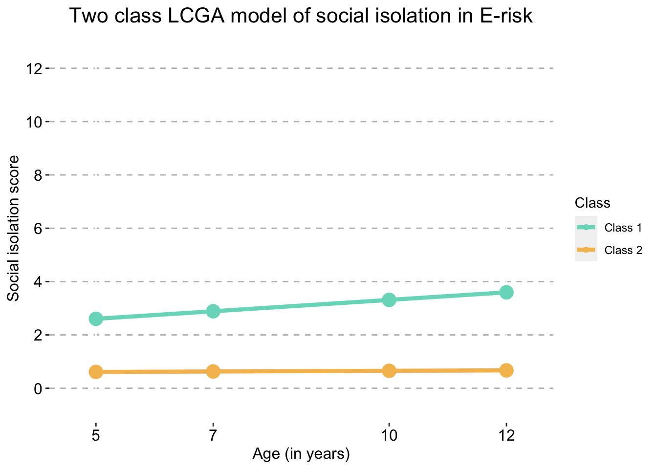
Three Class model
#create three class data frame with means and variances
three_class_si <- as.data.frame(
  si.classes.all$X.Users.katiethompson.Documents.PhD.LISS.DTP_Louise_and_Tim.Social.isolation.trajectories_Paper.1.data_analysis.mplus.LCGA.clustered.full_sample.output..LCGA_isolation_3traj_full_sample_clustered.out$gh5$means_and_variances_data$y_estimated_means)

#name the variables
names(three_class_si) <- c("Class 1","Class 2","Class 3")

#create time point column
three_class_si$timepoint <- c(5, 7, 10, 12)

#convert data to long format
three_class_si <- three_class_si %>%
  pivot_longer(-timepoint,
               names_to = "Class",
               values_to = "social.isolation_score")

#check
#three_class_si
three_traj_plot_clustered_full_sample <- ggplot(three_class_si,
aes(x = timepoint,
y = social.isolation_score,
colour = Class)) +
geom_line(size = 1.5) +
geom_point(aes(size = 1)) +
scale_fill_manual(values = palette3) +
scale_color_manual(values = palette3) +
labs(x = "Age (in years)",
title = "Three class LCGA model of social isolation in E-risk",
color = "Class",
y ="Social isolation score") +
scale_y_continuous(expand = c(0.1,0.1),
limits = c(0,12),
breaks = seq(0, 12, 2)) +
scale_x_continuous(expand = c(0.1,0.1),
limits = c(5,12),
breaks = c(5, 7, 10, 12)) +
theme(panel.grid.major.y = element_line(size = 0.5,
linetype = 'dashed',
colour = "gray"),
axis.text = element_text(colour="black",
size = 12),
axis.title = element_text(colour="black",
size = 12),
panel.background = element_blank(),
plot.title = element_text(size = 16, hjust=0.5)) +
guides(shape = FALSE, size = FALSE)
three_traj_plot_clustered_full_sample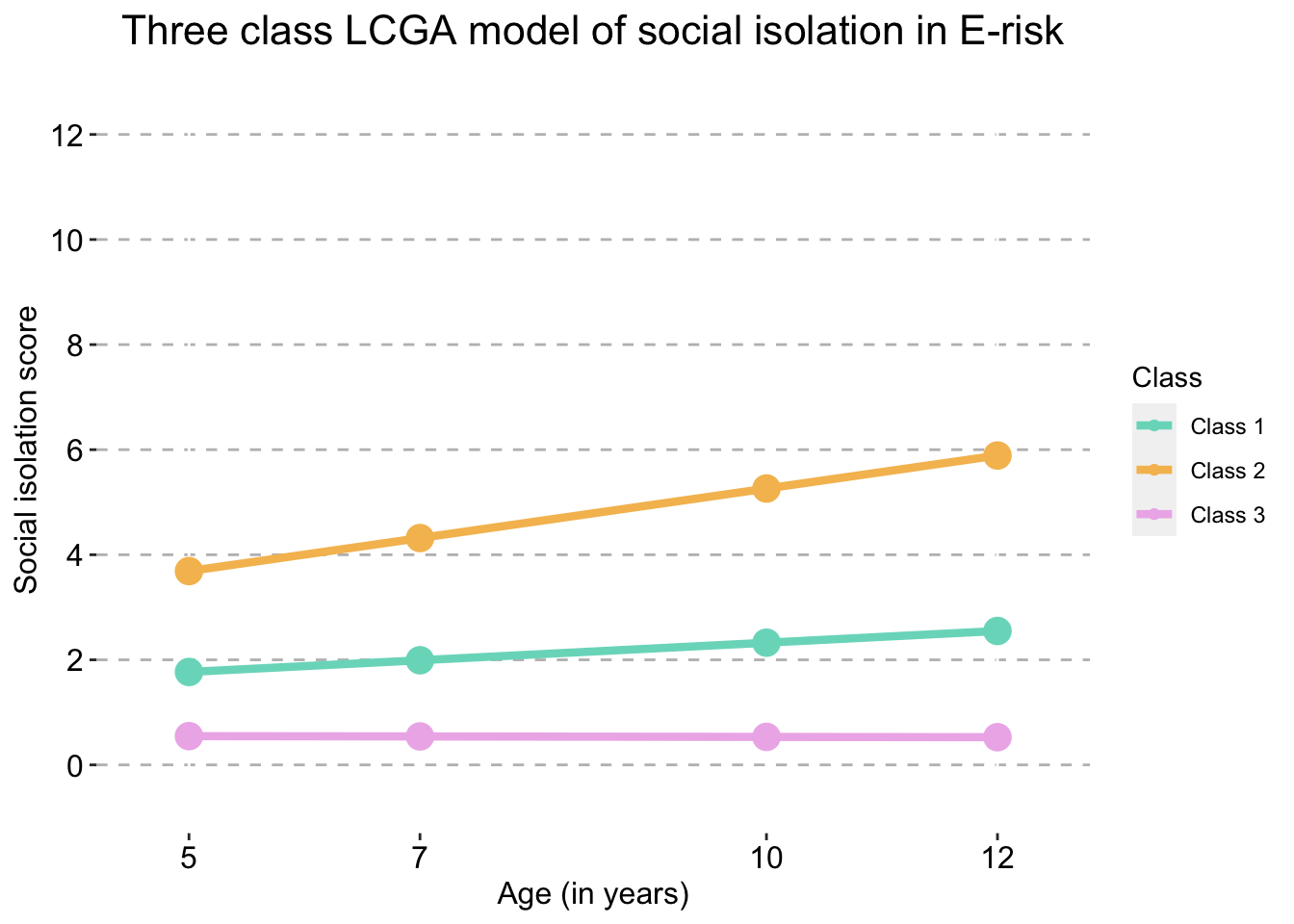
Four Class model
#create four class data frame with means and variances
four_class_si <- as.data.frame(
  si.classes.all$X.Users.katiethompson.Documents.PhD.LISS.DTP_Louise_and_Tim.Social.isolation.trajectories_Paper.1.data_analysis.mplus.LCGA.clustered.full_sample.output..LCGA_isolation_4traj_full_sample_clustered.out$gh5$means_and_variances_data$y_estimated_means)

#name the variables
names(four_class_si) <- c("Class 1","Class 2","Class 3","Class 4")

#create timepoint column
four_class_si$timepoint <- c(5, 7, 10, 12)

#convert data to long format
four_class_si <- four_class_si %>%
  pivot_longer(-timepoint,
               names_to = "Class",
               values_to = "social.isolation_score")

#check
#four_class_si
four_traj_plot_clustered_full_sample <- ggplot(four_class_si,
aes(x = timepoint,
y = social.isolation_score,
colour = Class)) +
geom_line(size = 1.5) +
geom_point(aes(size = 1)) +
scale_fill_manual(values = palette4) +
scale_color_manual(values = palette4) +
labs(x = "Age (in years)",
title = "Four class LCGA model of social isolation in E-risk",
color = "Class",
y ="Social isolation score") +
scale_y_continuous(expand = c(0.1,0.1),
limits = c(0,12),
breaks = seq(0, 12, 2)) +
scale_x_continuous(expand = c(0.1,0.1),
limits = c(5,12),
breaks = c(5, 7, 10, 12)) +
theme(panel.grid.major.y = element_line(size = 0.5,
linetype = 'dashed',
colour = "gray"),
axis.text = element_text(colour="black",
size = 12),
axis.title = element_text(colour="black",
size = 12),
panel.background = element_blank(),
plot.title = element_text(size = 16, hjust=0.5)) +
guides(shape = FALSE, size = FALSE)
four_traj_plot_clustered_full_sample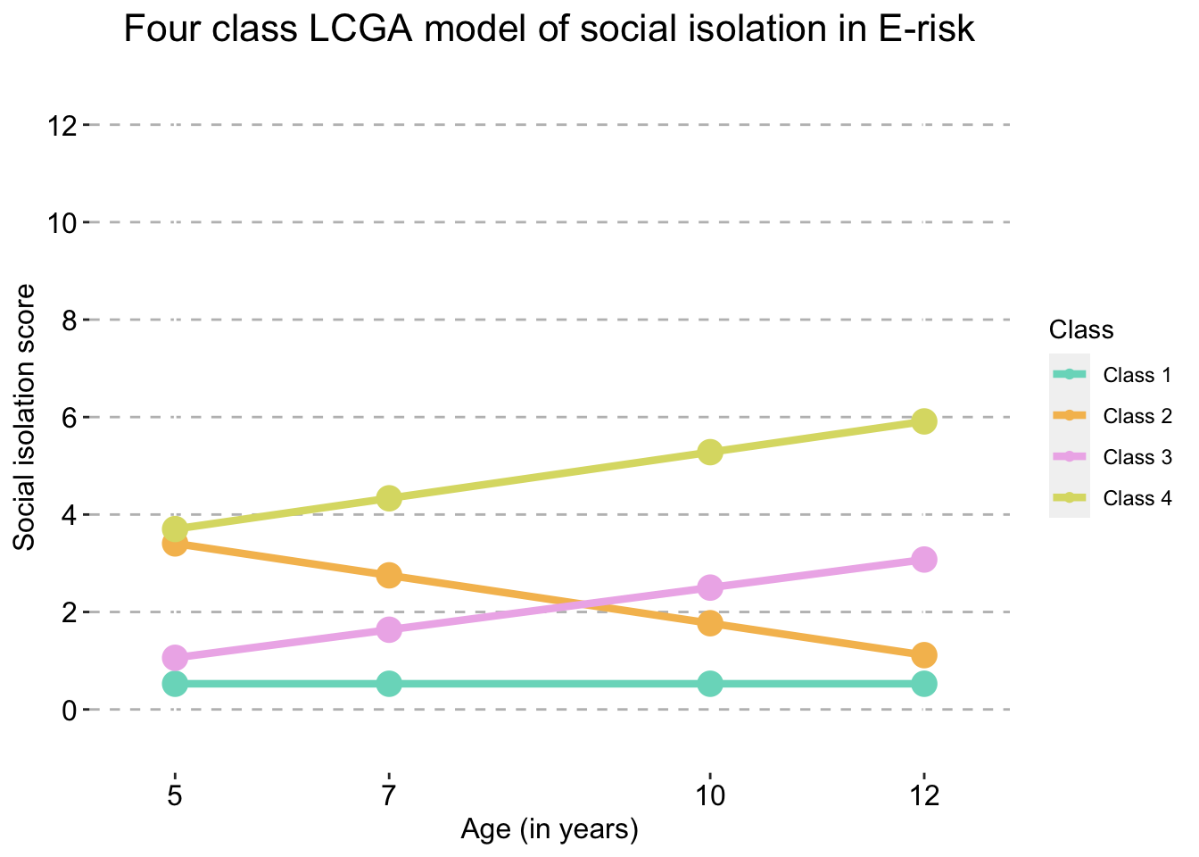
Five Class model
#create five class data frame with means and variances
five_class_si <- as.data.frame(
  si.classes.all$X.Users.katiethompson.Documents.PhD.LISS.DTP_Louise_and_Tim.Social.isolation.trajectories_Paper.1.data_analysis.mplus.LCGA.clustered.full_sample.output..LCGA_isolation_5traj_full_sample_clustered.out$gh5$means_and_variances_data$y_estimated_means)

#name the variables
names(five_class_si) <- c("Class 1","Class 2","Class 3","Class 4","Class 5")

#create timepoint column
five_class_si$timepoint <- c(5, 7, 10, 12)

#convert data to long format
five_class_si <- five_class_si %>%
  pivot_longer(-timepoint,
               names_to = "Class",
               values_to = "social.isolation_score")

#check
#five_class_si
five_traj_plot_clustered_full_sample <- ggplot(five_class_si,
aes(x = timepoint,
y = social.isolation_score,
colour = Class)) +
geom_line(size = 1.5) +
geom_point(aes(size = 1)) +
scale_fill_manual(values = palette5) +
scale_color_manual(values = palette5) +
labs(x = "Age (in years)",
title = "Five class LCGA model of social isolation in E-risk",
color = "Class",
y ="Social isolation score") +
scale_y_continuous(expand = c(0.1,0.1),
limits = c(0,12),
breaks = seq(0, 12, 2)) +
scale_x_continuous(expand = c(0.1,0.1),
limits = c(5,12),
breaks = c(5, 7, 10, 12)) +
theme(panel.grid.major.y = element_line(size = 0.5,
linetype = 'dashed',
colour = "gray"),
axis.text = element_text(colour="black",
size = 12),
axis.title = element_text(colour="black",
size = 12),
panel.background = element_blank(),
plot.title = element_text(size = 16, hjust=0.5)) +
guides(shape = FALSE, size = FALSE)
five_traj_plot_clustered_full_sample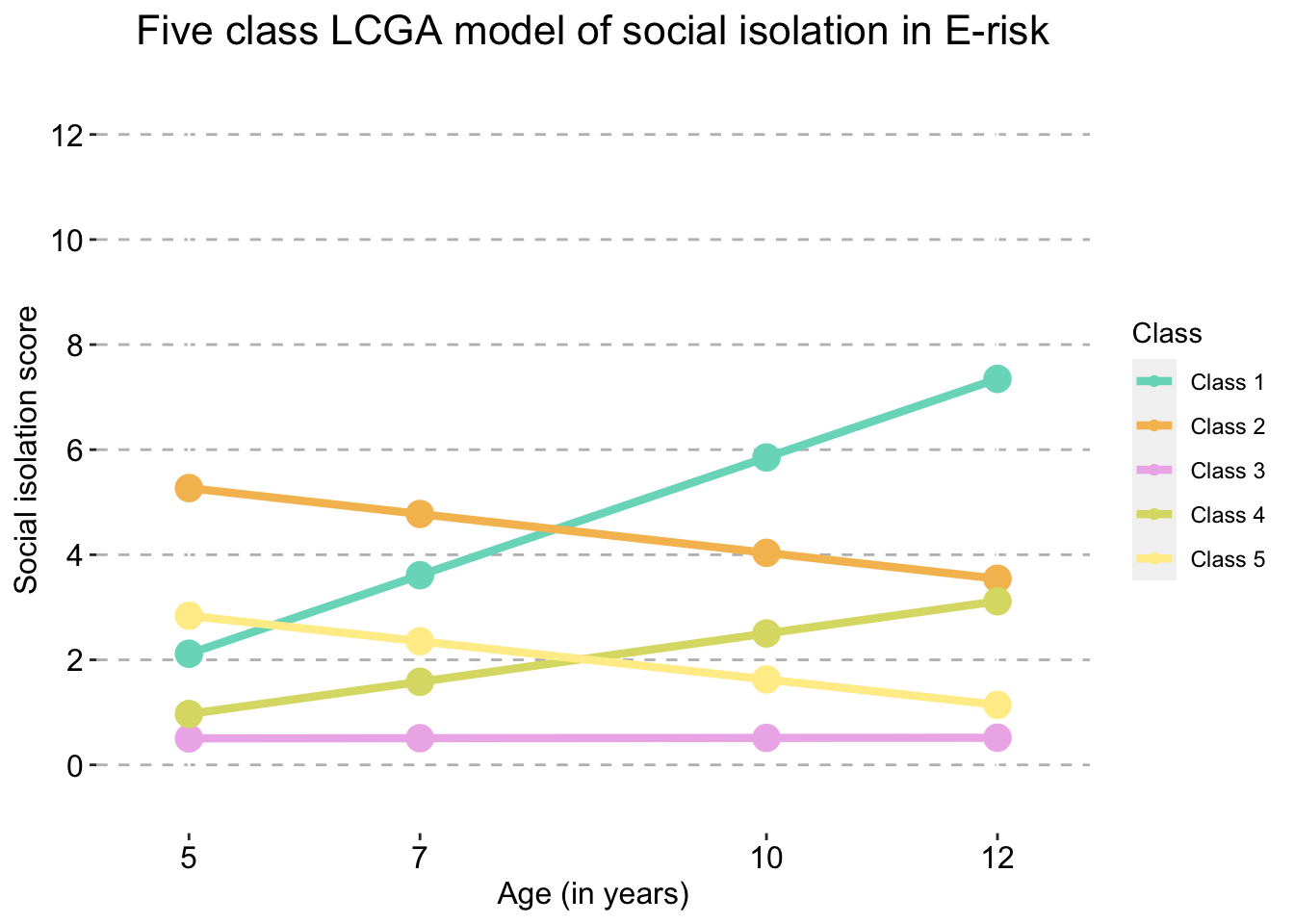
Six Class model
#create five class data frame with means and variances
six_class_si <- as.data.frame(
  si.classes.all$X.Users.katiethompson.Documents.PhD.LISS.DTP_Louise_and_Tim.Social.isolation.trajectories_Paper.1.data_analysis.mplus.LCGA.clustered.full_sample.output..LCGA_isolation_6traj_full_sample_clustered.out$gh5$means_and_variances_data$y_estimated_means)

#name the variables
names(six_class_si) <- c("Class 1","Class 2","Class 3","Class 4","Class 5","Class 6")

#create timepoint column
six_class_si$timepoint <- c(5, 7, 10, 12)

#convert data to long format
six_class_si <- six_class_si %>%
  pivot_longer(-timepoint,
               names_to = "Class",
               values_to = "social.isolation_score")

#check
#six_class_si
six_traj_plot_clustered_full_sample <- ggplot(six_class_si,
aes(x = timepoint,
y = social.isolation_score,
colour = Class)) +
geom_line(size = 1.5) +
geom_point(aes(size = 1)) +
scale_fill_manual(values = palette6) +
scale_color_manual(values = palette6) +
labs(x = "Age (in years)",
title = "Six class LCGA model of social isolation in E-risk",
color = "Class",
y = "Social isolation score") +
scale_y_continuous(expand = c(0.1,0.1),
limits = c(0,12),
breaks = seq(0, 12, 2)) +
scale_x_continuous(expand = c(0.1,0.1),
limits = c(5,12),
breaks = c(5, 7, 10, 12)) +
theme(panel.grid.major.y = element_line(size = 0.5,
linetype = 'dashed',
colour = "gray"),
axis.text = element_text(colour="black",
size = 12),
axis.title = element_text(colour="black",
size = 12),
panel.background = element_blank(),
plot.title = element_text(size = 16, hjust=0.5)) +
guides(shape = FALSE, size = FALSE)
six_traj_plot_clustered_full_sample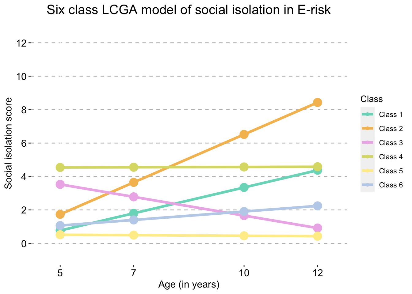
Combined LCGA trajectory plot
#combine all plots
library(ggpubr) # Needed for combining plots
library(gridExtra)
combined_trajectories_plot_clustered_full_sample <- ggarrange(
                                        two_traj_plot_clustered_full_sample,
                                        three_traj_plot_clustered_full_sample,
                                        four_traj_plot_clustered_full_sample,
                                        five_traj_plot_clustered_full_sample,
                                        six_traj_plot_clustered_full_sample,
                                        ncol = 2, nrow = 3,
                                        widths = c(2.7,2.7,2.7,2.7),
                                        heights = c(3,3,3,3),
                                        labels = c("A", "B", "C", "D", "E", "F"),
                                        legend = "bottom")

# ggsave(
#   "LCGA_combined_trajectories_plot_clustered_full_sample.jpeg",
#   plot = combined_trajectories_plot_clustered_full_sample,
#   device = "jpeg",
#   path = paste0(graph_save_data_path, "LCGA/"),
#   width = 9,
#   height = 10
# )
combined_trajectories_plot_clustered_full_sample
Work by Katherine N Thompson
katherine.n.thompson@kcl.ac.uk