#source raw data directory: data_raw and data included
source("../../../isolation_trajectories_data_path.R")

Quadratic GMM

Quadratic term significance for each model

si.quad.all <- readModels(paste0(mplus_GMM_clustered_full_output_QUAD_data_path), recursive = TRUE)

#extract the summary variables from the mplus output files. Assuming there are multiple files in the above directory, model summaries could be retained as a data.frame as follows:
si_quad_summaries <- do.call("rbind.fill",
                        sapply(si.quad.all,
                               "[", 
                               "summaries"))

Here we only reprt trsults for the two and three class models as the four to six class models did not converge.

4th class originally had problems with negative S variances - set S@0 for this model, this then resulted in non-convergence.
5th class originally had problems with negative S variances - set S@0 for this model, this then resulted in non-convergence.
6th class originally had problems with negative S variances - set S@0 for this model, this then resulted in non-convergence.

Significance values for 2 class model: Q has significant mean for class 1 (0.044), although only just. Q has non significant mean for class 2 (0.085).

Significance values for 3 class model: Q has significant mean for class 1 (0.001). Q has significant mean for class 2 (0.002). Q has significant mean for class 3 (0.008).

# two class
quad.mean.two.class <- si.quad.all$X.Users.katiethompson.Documents.PhD.LISS.DTP_Louise_and_Tim.Social.isolation.trajectories_Paper.1.data_analysis.mplus.GMM.clustered.full_sample.quadratic..isolation_2traj_full_sample_clustered_QUAD.out$parameters$unstandardized %>%
  filter(paramHeader == "Means" & LatentClass < 7) # filter out the means for I, S and Q for each class 

quad.variance.two.class <- si.quad.all$X.Users.katiethompson.Documents.PhD.LISS.DTP_Louise_and_Tim.Social.isolation.trajectories_Paper.1.data_analysis.mplus.GMM.clustered.full_sample.quadratic..isolation_2traj_full_sample_clustered_QUAD.out$parameters$unstandardized %>%
  filter(paramHeader == "Variances" & LatentClass < 7) # filter out the means for I, S and Q for each class 

# three class
quad.mean.three.class <- si.quad.all$X.Users.katiethompson.Documents.PhD.LISS.DTP_Louise_and_Tim.Social.isolation.trajectories_Paper.1.data_analysis.mplus.GMM.clustered.full_sample.quadratic..isolation_3traj_full_sample_clustered_QUAD.out$parameters$unstandardized %>%
  filter(paramHeader == "Means" & LatentClass < 7) # filter out the means for I, S and Q for each class 

quad.variance.three.class <- si.quad.all$X.Users.katiethompson.Documents.PhD.LISS.DTP_Louise_and_Tim.Social.isolation.trajectories_Paper.1.data_analysis.mplus.GMM.clustered.full_sample.quadratic..isolation_3traj_full_sample_clustered_QUAD.out$parameters$unstandardized %>%
  filter(paramHeader == "Variances" & LatentClass < 7) # filter out the means for I, S and Q for each class

Two class model

two.class.mean.var <- rbind(quad.mean.two.class, quad.variance.two.class) %>%
  select(`Mean/variance` = paramHeader, 
         `Intercept/slope/quadratic` = param, 
         `estimate` = est, 
         `standard error` = se, 
         `p value` = pval)
kable(two.class.mean.var)

Mean/variance	Intercept/slope/quadratic	estimate	standard error	p value
Means	I	0.714	0.030	0.000
Means	S	0.033	0.022	0.127
Means	Q	-0.006	0.003	0.044
Means	I	1.979	0.227	0.000
Means	S	-0.087	0.254	0.732
Means	Q	0.067	0.039	0.085
Variances	I	0.642	0.119	0.000
Variances	S	0.081	0.029	0.006
Variances	Q	0.001	0.001	0.013
Variances	I	0.642	0.119	0.000
Variances	S	0.081	0.029	0.006
Variances	Q	0.001	0.001	0.013

Three class model

three.class.mean.var <- rbind(quad.mean.three.class, quad.variance.three.class) %>%
  select(`Mean/variance` = paramHeader, 
         `Intercept/slope/quadratic` = param, 
         `estimate` = est, 
         `standard error` = se, 
         `p value` = pval)
kable(three.class.mean.var)

Mean/variance	Intercept/slope/quadratic	estimate	standard error	p value
Means	I	0.594	0.041	0.000
Means	S	0.078	0.023	0.001
Means	Q	-0.010	0.003	0.001
Means	I	1.417	0.223	0.000
Means	S	-0.142	0.207	0.493
Means	Q	0.095	0.031	0.002
Means	I	4.274	0.638	0.000
Means	S	-0.826	0.202	0.000
Means	Q	0.069	0.026	0.008
Variances	I	0.244	0.095	0.010
Variances	S	0.073	0.028	0.010
Variances	Q	0.001	0.000	0.014
Variances	I	0.244	0.095	0.010
Variances	S	0.073	0.028	0.010
Variances	Q	0.001	0.000	0.014
Variances	I	0.244	0.095	0.010
Variances	S	0.073	0.028	0.010
Variances	Q	0.001	0.000	0.014

Model fit statistics for two and three class models

# remove 4,5,6 class models
si.two_three.summaries <- si_quad_summaries[-c(3:5),]

#social isolation summaries 
si.class.summaries <- data.frame(matrix(nrow = 2, 
                                         ncol = 8)) 

#create column names for the variables you will be adding to the empty matrix of si.class.summaries
colnames(si.class.summaries) <- c("Model", 
                                  "Parameters", 
                                  "AIC", 
                                  "BIC", 
                                  "aBIC", 
                                  "Entropy", 
                                  "VLMR LRT p-value", 
                                  "Class Proportions") #or whichever indices you want to compare; do si_summaries$ to see what's in there

#check colnames
#si.class.summaries

#create "Model" variable
si.class.summaries <- si.class.summaries %>%
  mutate(
    Model = 
    as.factor(c("Two Class", #change nrow in data frame above when adding more models
                "Three Class")))  

#add summary information into data frame 
si.class.summaries <- si.class.summaries %>%
  mutate(
    Parameters = 
      si.two_three.summaries$Parameters) %>% #parameters col from original summaries data set
  mutate(
    AIC = 
      si.two_three.summaries$AIC) %>% #AIC col from original summaries data set
  mutate(
    BIC = 
      si.two_three.summaries$BIC) %>% #BIC col from original summaries data set
  mutate(
    aBIC = 
      si.two_three.summaries$aBIC) %>% #aBIC col from original summaries data set
  mutate(
    Entropy = 
      si.two_three.summaries$Entropy) %>% #Entropy col from original summaries data set
  mutate(
    `VLMR LRT p-value` = 
      si.two_three.summaries$T11_VLMR_PValue) #T11_VLMR_PValue col from original summaries data set

#check
#si.class.summaries

#for each class we want to add in the model estimated class counts - then convert this into a list with the percentage of people in each class

#two classes
si.class.summaries$`Class Proportions`[si.class.summaries$Model == "Two Class"] <- list(c(sprintf("%.0f", si.quad.all$X.Users.katiethompson.Documents.PhD.LISS.DTP_Louise_and_Tim.Social.isolation.trajectories_Paper.1.data_analysis.mplus.GMM.clustered.full_sample.quadratic..isolation_2traj_full_sample_clustered_QUAD.out$class_counts$modelEstimated$proportion*100)))

#three classes
si.class.summaries$`Class Proportions`[si.class.summaries$Model == "Three Class"] <- list(c(sprintf('%.0f', si.quad.all$X.Users.katiethompson.Documents.PhD.LISS.DTP_Louise_and_Tim.Social.isolation.trajectories_Paper.1.data_analysis.mplus.GMM.clustered.full_sample.quadratic..isolation_3traj_full_sample_clustered_QUAD.out$class_counts$modelEstimated$proportion*100)))

#two classes
si.class.summaries$`Class N`[si.class.summaries$Model == "Two Class"] <- list(c(sprintf("%.0f", si.quad.all$X.Users.katiethompson.Documents.PhD.LISS.DTP_Louise_and_Tim.Social.isolation.trajectories_Paper.1.data_analysis.mplus.GMM.clustered.full_sample.quadratic..isolation_2traj_full_sample_clustered_QUAD.out$class_counts$posteriorProb$count)))

#three classes
si.class.summaries$`Class N`[si.class.summaries$Model == "Three Class"] <- list(c(sprintf("%.0f", si.quad.all$X.Users.katiethompson.Documents.PhD.LISS.DTP_Louise_and_Tim.Social.isolation.trajectories_Paper.1.data_analysis.mplus.GMM.clustered.full_sample.quadratic..isolation_3traj_full_sample_clustered_QUAD.out$class_counts$posteriorProb$count)))

#Look at summary table 
kable(si.class.summaries)

Model	Parameters	AIC	BIC	aBIC	Entropy	VLMR LRT p-value	Class Proportions	Class N
Two Class	17	25392.55	25489.63	25435.62	0.950	0.0562	93, 7	2071, 161
Three Class	21	24762.68	24882.60	24815.88	0.956	0.2802	90, 5 , 5	2014, 114 , 104

Plots

Two Class model

#create two class data frame with means and variances
two_class_si <- as.data.frame(
  si.quad.all$X.Users.katiethompson.Documents.PhD.LISS.DTP_Louise_and_Tim.Social.isolation.trajectories_Paper.1.data_analysis.mplus.GMM.clustered.full_sample.quadratic..isolation_2traj_full_sample_clustered_QUAD.out$gh5$means_and_variances_data$y_estimated_means)

#name the variables
names(two_class_si) <- c("Class 1","Class 2")

#create time point column 
two_class_si$timepoint <- c(5, 7, 10, 12)

#convert data to long format 
two_class_si <- two_class_si %>%
  pivot_longer(-timepoint, 
               names_to = "Class", 
               values_to = "social.isolation_score")

#check
#two_class_si

two_traj_plot_clustered_full_sample <- ggplot(two_class_si,
        aes(x = timepoint, 
            y = social.isolation_score, 
            colour = Class)) +
          geom_line(size = 1.5) +
  geom_point(aes(#shape = class, 
                 size = 1)) +
  scale_fill_manual(values = palette2) +
  scale_color_manual(values = palette2) +
  labs(x = "Age (in years)", 
       title = "Two class model",
       color = "Class",
       y ="Social isolation score") +   
  scale_y_continuous(expand = c(0.1,0.1),
                     limits = c(0,12),
                     breaks = seq(0, 12, 2)) +
  scale_x_continuous(expand = c(0.1,0.1),
                     limits = c(5,12),
                     breaks = c(5, 7, 10, 12)) +
  theme(panel.grid.major.y = element_line(size = 0.5,
                                        linetype = 'dashed',
                                        colour = "gray"),
        axis.text = element_text(colour="black", 
                                 size = 12),
        axis.title = element_text(colour="black", 
                                  size = 12),
        panel.background = element_blank(),
        plot.title = element_text(size = 16, hjust = 0.5)) + 
  guides(shape = FALSE, size = FALSE)

two_traj_plot_clustered_full_sample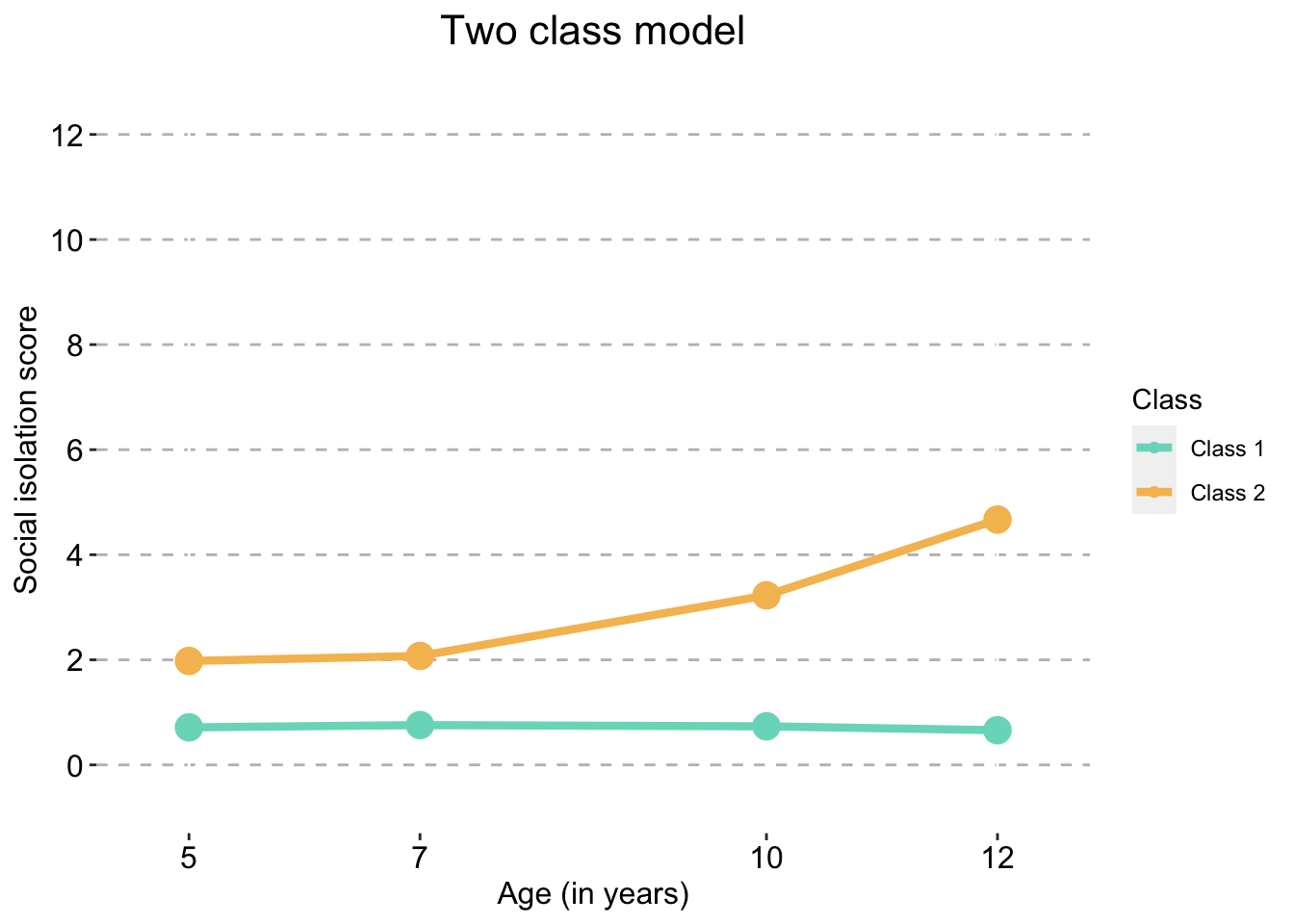

Three Class model

#create three class data frame with means and variances
three_class_si <- as.data.frame(
  si.quad.all$X.Users.katiethompson.Documents.PhD.LISS.DTP_Louise_and_Tim.Social.isolation.trajectories_Paper.1.data_analysis.mplus.GMM.clustered.full_sample.quadratic..isolation_3traj_full_sample_clustered_QUAD.out$gh5$means_and_variances_data$y_estimated_means)

#name the variables
names(three_class_si) <- c("Class 1","Class 2","Class 3")

#create time point column 
three_class_si$timepoint <- c(5, 7, 10, 12)

#convert data to long format 
three_class_si <- three_class_si %>%
  pivot_longer(-timepoint, 
               names_to = "Class", 
               values_to = "social.isolation_score")

#check
#three_class_si

three_traj_plot_clustered_full_sample <- ggplot(three_class_si,
        aes(x = timepoint, 
            y = social.isolation_score, 
            colour = Class)) +
          geom_line(size = 1.5) +
  geom_point(aes(size = 1)) +
  scale_fill_manual(values = palette3) +
  scale_color_manual(values = palette3) +
  labs(x = "Age (in years)", 
       title = "Three class model",
       color = "Class",
       y ="Social isolation score") +   
  scale_y_continuous(expand = c(0.1,0.1),
                     limits = c(0,12),
                     breaks = seq(0, 12, 2)) +
  scale_x_continuous(expand = c(0.1,0.1),
                     limits = c(5,12),
                     breaks = c(5, 7, 10, 12)) +
  theme(panel.grid.major.y = element_line(size = 0.5,
                                        linetype = 'dashed',
                                        colour = "gray"),
        axis.text = element_text(colour="black", 
                                 size = 12),
        axis.title = element_text(colour="black", 
                                  size = 12),
        panel.background = element_blank(),
        plot.title = element_text(size = 16, hjust=0.5)) + 
  guides(shape = FALSE, size = FALSE)

three_traj_plot_clustered_full_sample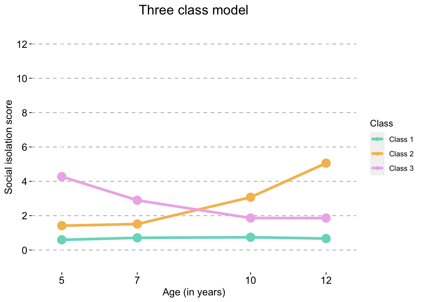

Allocation differences between linear and quadratic 3 class model

dat.descriptives <- readRDS(file = paste0(data_path, "preprocessed_isolation_trajectories_Jan2021_full_sample.rds"))
#colnames(dat.descriptives)

dat.tra.prob.full.LINEAR <- read.table(paste0(mplus_GMM_clustered_full_output_data_path, "GMM_SI_3Cl_full_sample_clustered.txt"), 
                            header = FALSE, 
                            col.names = c("SISOE5", # original social isolation score at age 5
                                         "SISOE7",  # original social isolation score at age 7
                                         "SISOE10", # original social isolation score at age 10
                                         "SISOE12", # original social isolation score at age 12
                                         "I",       # intercept
                                         "S",       # slope
                                         "C_I",     # factor scores based on most likely class membership
                                         "C_S",     # factor scores based on most likely class membership
                                         "CPROB1",  # class probability 1
                                         "CPROB2",  # class probability 2
                                         "CPROB3",  # class probability 3
                                         "C",       # class 
                                         "ID",      # ID
                                         "FAMILYID" # Family ID - twin clustering  
                                       ))   
#check 
#dat.tra.prob.full.LINEAR

dat.tra.prob.full.QUAD <- read.table(paste0(mplus_GMM_clustered_full_output_QUAD_data_path, "GMM_SI_3Cl_full_sample_clustered_QUAD.txt"), 
                            header = FALSE, 
                            col.names = c("SISOE5", # original social isolation score at age 5
                                         "SISOE7",  # original social isolation score at age 7
                                         "SISOE10", # original social isolation score at age 10
                                         "SISOE12", # original social isolation score at age 12
                                         "I",       # intercept
                                         "S",       # slope
                                         "Q",       # quadratic
                                         "C_I",     # factor scores based on most likely class membership
                                         "C_S",     # factor scores based on most likely class membership
                                         "C_Q",     # factor scores based on most likely class membership
                                         "CPROB1",  # class probability 1
                                         "CPROB2",  # class probability 2
                                         "CPROB3",  # class probability 3
                                         "C",       # class 
                                         "ID",      # ID
                                         "FAMILYID" # Family ID - twin clustering  
                                       ))   
#check 
#dat.tra.prob.full.QUAD

dat.tra.prob.LINEAR <- dat.tra.prob.full.LINEAR %>%
  select(id = ID, 
         prob1.linear = CPROB1,
         prob2.linear = CPROB2,
         prob3.linear = CPROB3,
         class.linear = C
         )
#check 
#dat.tra.prob.LINEAR

dat.tra.prob.QUAD <- dat.tra.prob.full.QUAD %>%
  select(id = ID, 
         prob1.quad = CPROB1,
         prob2.quad = CPROB2,
         prob3.quad = CPROB3,
         class.quad = C
         )
#check 
#dat.tra.prob.QUAD

#create list of data frames to merge
dataframe_list <- list(
  dat.descriptives,
  dat.tra.prob.LINEAR,
  dat.tra.prob.QUAD
)

#merge data frames
dat <- plyr::join_all(
  dataframe_list,
  by = "id" # Alternatively you can join by several columns
  )

#check
#colnames(dat)

# linear
dat <- dat %>%
  mutate(class_renamed.linear =
    recode_factor(class.linear,
      "1" = "Low stable",
      "2" = "Increasing",
      "3" = "Decreasing"
    )
  )
as.data.frame(table(dat$class_renamed.linear)) %>% 
  select(`Linear classes` = Var1,
         Freq)

# quadratic
dat <- dat %>%
  mutate(class_renamed.quad =
    recode_factor(class.quad,
      "1" = "Low stable",
      "2" = "Increasing",
      "3" = "Decreasing"
    )
  )
as.data.frame(table(dat$class_renamed.quad)) %>% 
  select(`Quadratic classes` = Var1,
         Freq)

Matching classification

96.51% of people were classified the same way regardless if the model was linear or quadratic.

Overall average movement from Linear to Quadratic:

1 more person in the increasing class
18 less people in the decreasing class
17 more people in the low stable class

dat <- dat %>%
  mutate(
    matching.class = 
      case_when(
        class.linear == class.quad ~ "Matching",
        class.linear != class.quad ~ "Not matching"
      )
  )

freq(dat$matching.class,
        cumul = FALSE, 
       display.type = FALSE, 
       headings = FALSE,
       style = "rmarkdown",
       report.nas = FALSE)

	Freq	%
Matching	2154	96.51
Not matching	78	3.49
Total	2232	100.00

29 in the decreasing class changed classes in the quadratic model.
19 in the increasing class changed classes in the quadratic model.
30 in the low stable class changed classes in the quadratic model. == 78 who are not matching.

dat <- dat %>%
  mutate(matching.isolated =
           case_when(
             matching.class == "Matching" & class_renamed.linear == "Increasing" ~ "Matching and increasing",
             matching.class == "Matching" & class_renamed.linear == "Decreasing" ~ "Matching and decreasing",
             matching.class == "Matching" & class_renamed.linear == "Low stable" ~ "Matching and low stable"
           ))

freq(dat$matching.isolated,
        cumul = FALSE, 
       display.type = FALSE, 
       headings = FALSE,
       style = "rmarkdown",
       report.nas = FALSE)

	Freq	%
Matching and decreasing	88	4.09
Matching and increasing	87	4.04
Matching and low stable	1979	91.88
Total	2154	100.00

dat.non.match <- dat %>%
  filter(matching.class == "Not matching")

# from linear to quadratic model
dat.non.match <- dat.non.match %>%
  mutate(
    direction.match =
      case_when(
        class_renamed.linear == "Increasing" & class_renamed.quad == "Low stable" ~ "Increasing to low stable",
        class_renamed.linear == "Decreasing" & class_renamed.quad == "Low stable" ~ "Decreasing to low stable",
        class_renamed.linear == "Increasing" & class_renamed.quad == "Decreasing" ~ "Increasing to decreasing",
        class_renamed.linear == "Decreasing" & class_renamed.quad == "Increasing" ~ "Decreasing to increasing",
        class_renamed.linear == "Low stable" & class_renamed.quad == "Increasing" ~ "Low stable to increasing",
        class_renamed.linear == "Low stable" & class_renamed.quad == "Decreasing" ~ "Low stable to decreasing",
      )
  )

freq(dat.non.match$direction.match,
     cumul = FALSE, 
       display.type = FALSE, 
       headings = FALSE,
       style = "rmarkdown",
       report.nas = FALSE)

	Freq	%
Decreasing to increasing	1	1.28
Decreasing to low stable	28	35.90
Increasing to low stable	19	24.36
Low stable to decreasing	11	14.10
Low stable to increasing	19	24.36
Total	78	100.00

1 person moved from the decreasing to the increasing class.
28 people moved from the decreasing to the low stable class.
19 people moved from the increasing to the low stable class.
11 people moved from the low stable to the decreasing class.
19 people moved from the low stable to the increasing class. == 78 non matching.

Work by Katherine N Thompson

katherine.n.thompson@kcl.ac.uk

GMM trajectory statistics and figures for quadratic models