Main analyses
# save R data file
saveRDS(object = dat, file = paste0(data_path, "class_joined_preprocessed_isolation_data_full_sample.rds"))This page contains the code to combine the original Rmd dataset and the new Mplus output. We also include relevant descriptive statistics for the classes/trajectories. We have used the hard classification variable given by Mplus for our analyses. We conduct sensitivity analyses using the 3STEP approach, data is prepped for this at the end of this page. Please note, if you are running this analysis for yourself, you will need to do this step after running your Mplus models and before analysing the data in Rmd
We have read in the processed R data and the Mplus model information to show who is has identified into which class.
dat.descriptives <- readRDS(file = paste0(data_path, "preprocessed_isolation_trajectories_Jan2021_full_sample.rds"))The Mplus output file contains the raw original data, slope estimate, intercept estimate, factor scores based on the slope and intercept, class probabilities for each person per class, and the hard class classification.
dat.tra.prob.full <- read.table(paste0(mplus_GMM_clustered_full_output_data_path, "GMM_SI_3Cl_full_sample_clustered.txt"),
                            header = FALSE,
                            col.names = c("SISOE5", # original social isolation score at age 5
                                         "SISOE7",  # original social isolation score at age 7
                                         "SISOE10", # original social isolation score at age 10
                                         "SISOE12", # original social isolation score at age 12
                                         "I",       # intercept
                                         "S",       # slope
                                         "C_I",     # factor scores based on most likely class membership
                                         "C_S",     # factor scores based on most likely class membership
                                         "CPROB1",  # class probability 1
                                         "CPROB2",  # class probability 2
                                         "CPROB3",  # class probability 3
                                         "C",       # class
                                         "ID",      # ID
                                         "FAMILYID" # Family ID - twin clustering
                                       ))
#check
head(dat.tra.prob.full)
We will only need the classification probabilities and the hard classification variable. This is then combined with the rest of our Rmd data.
dat.tra.prob <- dat.tra.prob.full %>%
  select(id = ID,
         prob1 = CPROB1,
         prob2 = CPROB2,
         prob3 = CPROB3,
         class = C
         )
#check
# dat.tra.prob

#create list of data frames to merge
dataframe_list <- list(
  dat.descriptives,
  dat.tra.prob
)

#merge data frames
dat <- plyr::join_all(
  dataframe_list,
  by = "id" # Alternatively you can join by several columns
  )

#check
# colnames(dat)
The class variable is then renamed to reflect the pattern seen in the classes identified. Here, we name them “Low stable”, “Increasing”, and “Decreasing” to reflect the pattern of each of the linear curves.
dat <- dat %>%
  mutate(class_renamed =
    recode_factor(class,
      "1" = "Low stable",
      "2" = "Increasing",
      "3" = "Decreasing"
    )
  )

data.frame(table(dat$class_renamed))combined_social_isolation <- c("isolation_combined_05",
"isolation_combined_07",
"isolation_combined_10",
"isolation_combined_12")
#convert to long format
dat_long <- dat %>%
gather(
key = "time_point_raw",
value = "social_isolation",
all_of(combined_social_isolation)) %>%
select(
id,
sex,
time_point_raw,
social_isolation,
class_renamed)
#head(dat_long)
#create variable that has just the number for the time point
dat_long <- dat_long %>%
mutate(time_point =
recode_factor(time_point_raw,
"isolation_combined_05" = "5",
"isolation_combined_07" = "7",
"isolation_combined_10" = "10",
"isolation_combined_12" = "12")) %>%
select(
id,
sex,
time_point,
social_isolation,
class_renamed)
#head(dat_long)spaghetti_plot <- ggplot(data = dat_long,
aes(x = time_point,
y = social_isolation,
group = factor(id),
color = class_renamed)) +
geom_line() +
scale_color_manual(name = "Class", values = palette3) +
labs(y = "Social isolation score",
x = "Age (years)") +
scale_x_discrete(expand = c(0.05,0.05), breaks = c("5", "7", "10", "12")) +
scale_y_continuous(expand = c(0.05,0.05), breaks = c(0,2,4,6,8,10,12)) +
theme(
panel.grid.major.y = element_line(size = 0.2,linetype = 'dashed',colour = "gray"),
axis.title.x = element_text(size = 12,face="bold"),
axis.title.y = element_text(size = 12,face="bold"),
axis.text.x = element_text(colour = "black", size = 10),
axis.text.y = element_text(colour = "black", size = 10),
panel.background = element_blank(),
legend.position = "bottom")The trajectory of each participant is plotted separately and colour coded depending on which class they were classified. Decreasing is indicated in pink, Increasing in Orange, and Low stable in blue. The average class trajectories are then plotted over the top.
#For class models, read in all output files within your folder that you have all your class models
si.classes.all <- readModels(paste0(mplus_GMM_clustered_full_output_data_path), recursive = TRUE) #Recursive means it reads data in sub-folders too
#create three class data frame with means and variances
three_class_si <- as.data.frame(
si.classes.all$X.Users.katiethompson.Documents.PhD.LISS.DTP_Louise_and_Tim.Social.isolation.trajectories_Paper.1.data_analysis.mplus.GMM.clustered.full_sample.output..isolation_3traj_full_sample_clustered.out$gh5$means_and_variances_data$y_estimated_means)
#name the variables
names(three_class_si) <- c("Class 1","Class 2","Class 3")
#create time point column
three_class_si$time_point <- factor(c("5","7","10","12"))
#convert data to long format
three_class_si <- three_class_si %>%
pivot_longer(-time_point,
names_to = "class_renamed",
values_to = "social_isolation")
# create factor for Class variable
three_class_si <- three_class_si %>%
mutate(class_renamed =
factor(class_renamed,
levels = c("Class 1","Class 2","Class 3"))) spaghetti_plotB <- ggplot(data = dat_long,
aes(x = time_point,
y = social_isolation,
color = class_renamed)) +
geom_line(aes(group = factor(id)), alpha = 0.9, size = 0.5) +
geom_line(data = three_class_si, aes(group = class_renamed), size = 1, alpha = 1) +
scale_color_manual(name = "class_renamed", values = palette_spag) +
labs(y = "Social isolation score",
x = "Age (years)") +
scale_x_discrete(expand = c(0.05,0.05), breaks = c("5", "7", "10", "12")) +
scale_y_continuous(expand = c(0.05,0.05), breaks = c(0,2,4,6,8,10,12)) +
theme(
panel.grid.major.y = element_line(size = 0.2,linetype = 'dashed',colour = "gray"),
axis.title.x = element_text(size = 12,face="bold"),
axis.title.y = element_text(size = 12,face="bold"),
axis.text.x = element_text(colour = "black", size = 10),
axis.text.y = element_text(colour = "black", size = 10),
panel.background = element_blank(),
legend.position = "none")
spaghetti_plotB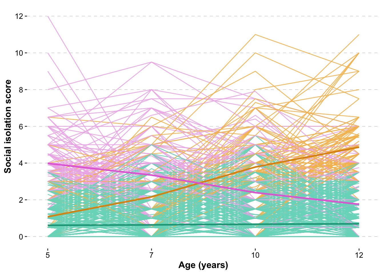
# ggsave(
#   "spaghetti_plot_three_class_colour_coded.jpeg",
#   plot = spaghetti_plotB,
#   device = "jpeg",
#   path = paste0(graph_save_data_path, "trajectories/"),
#   width = 7,
#   height = 5
# )The code to create these descriptives is long, so has been hidden here, please see raw code on Github if interested. The descriptives include ethnicity, SES, zygosity, and sex.
#final descriptives by class table
kable(class.descriptives)| Category | Descriptive | Low stable | % Low stable | Increasing | % Increasing | Decreasing | % Decreasing | Total | % Total |
|---|---|---|---|---|---|---|---|---|---|
| Sex | Male | 961 | 47.83 | 62 | 58.49 | 69 | 58.97 | 1092 | 48.92 |
| Female | 1048 | 52.17 | 44 | 41.51 | 48 | 41.03 | 1140 | 51.08 | |
| Zygosity | MZ | 1133 | 56.40 | 55 | 51.89 | 54 | 46.15 | 1242 | 55.65 |
| DZ | 876 | 43.60 | 51 | 48.11 | 63 | 53.85 | 990 | 44.35 | |
| SES | Low | 630 | 31.36 | 57 | 53.77 | 55 | 47.01 | 742 | 33.24 |
| Middle | 681 | 33.90 | 27 | 25.47 | 30 | 25.64 | 738 | 33.06 | |
| High | 698 | 34.74 | 22 | 20.75 | 32 | 27.35 | 752 | 33.69 | |
| Ethnicity | White | 1818 | 90.49 | 102 | 96.23 | 98 | 83.76 | 2018 | 90.41 |
| Asian | 78 | 3.88 | 2 | 1.89 | 10 | 8.55 | 90 | 4.03 | |
| Black | 36 | 1.79 | 0 | 0.00 | 6 | 5.13 | 42 | 1.88 | |
| Mixed race | 7 | 0.35 | 0 | 0.00 | 1 | 0.85 | 8 | 0.36 | |
| Other | 70 | 3.48 | 2 | 1.89 | 2 | 1.71 | 74 | 3.32 |
We need to relevel the class variable to use the Low Stable class as the reference group in all subsequent regression analyses.
library(nnet)
# relevel class_factor
dat <- dat %>%
  mutate(
    class_reordered =
      relevel(
        class_renamed,
        ref = "Low stable",
        first = TRUE, #levels in ref come first
        collapse = "+", #String used when constructing names for combined factor levels
        xlevels = TRUE #levels maintained even if not actually occurring

      )
)Next, we calculate the classification probabilities, class means and NAs per class.
For the diagonal, this represents the probability given that the an observation is a part of a specific latent class that you will classify it as said class.
Note this does not represent average probabilities as this table wasn’t available in Mplus version 8.
# extract the classification probabilities for the most likely class memberships (column) by latent class (row). This shows the uncertainty rate of the probabilities. If it was perfect - the diagonal would be 1. E.g. for Class 1 - 98.3% of individuals fit that category.
class.probs <- data.frame(class.all$X.Users.katiethompson.Documents.PhD.LISS.DTP_Louise_and_Tim.Social.isolation.trajectories_Paper.1.data_analysis.mplus.GMM.clustered.full_sample.output..isolation_3traj_full_sample_clustered.out$class_counts$classificationProbs.mostLikely)

# add column names
colnames(class.probs) <- c("Low stable","Increasing","Decreasing")

class.probs$Class <- c("Low stable","Increasing","Decreasing")

# as.tibble(class.probs)

class.probs <- class.probs %>%
  tidyr::pivot_longer(-Class,
               names_to = "class",
               values_to = "Classification probabilities")

class.probs <- class.probs[-c(2:4,6:8),-c(2)]kable(class.probs)| Class | Classification probabilities |
|---|---|
| Low stable | 0.989 |
| Increasing | 0.871 |
| Decreasing | 0.899 |
# extract means for each class
class.1.means <- as.tibble(class.all$X.Users.katiethompson.Documents.PhD.LISS.DTP_Louise_and_Tim.Social.isolation.trajectories_Paper.1.data_analysis.mplus.GMM.clustered.full_sample.output..isolation_3traj_full_sample_clustered.out$tech7$CLASS.1$classSampMeans)

class.2.means <- as.tibble(class.all$X.Users.katiethompson.Documents.PhD.LISS.DTP_Louise_and_Tim.Social.isolation.trajectories_Paper.1.data_analysis.mplus.GMM.clustered.full_sample.output..isolation_3traj_full_sample_clustered.out$tech7$CLASS.2$classSampMeans)

class.3.means <- as.tibble(class.all$X.Users.katiethompson.Documents.PhD.LISS.DTP_Louise_and_Tim.Social.isolation.trajectories_Paper.1.data_analysis.mplus.GMM.clustered.full_sample.output..isolation_3traj_full_sample_clustered.out$tech7$CLASS.3$classSampMeans)

class.means <- rbind(class.1.means,class.2.means,class.3.means)

class.means$Class <- c("Low stable","Increasing","Decreasing")

class.means <- class.means %>%
  select(
    Class,
    `Mean at age 5` = SISOE5,
    `Mean at age 7` = SISOE7,
    `Mean at age 10` = SISOE10,
    `Mean at age 12` = SISOE12
)kable(class.means)| Class | Mean at age 5 | Mean at age 7 | Mean at age 10 | Mean at age 12 |
|---|---|---|---|---|
| Low stable | 0.605 | 0.632 | 0.718 | 0.673 |
| Increasing | 1.291 | 1.848 | 3.545 | 5.027 |
| Decreasing | 3.984 | 3.374 | 2.347 | 1.771 |
ctable(dat$class_renamed, dat$na.per.person.si)Cross-Tabulation, Row Proportions
dat\(class_renamed * dat\)na.per.person.si
| dat$na.per.person.si | 0 | 1 | 2 | 3 | Total | |
| dat$class_renamed | ||||||
| Low stable | 1874 (93.3%) | 79 (3.9%) | 39 (1.9%) | 17 (0.8%) | 2009 (100.0%) | |
| Increasing | 97 (91.5%) | 6 (5.7%) | 3 (2.8%) | 0 (0.0%) | 106 (100.0%) | |
| Decreasing | 108 (92.3%) | 4 (3.4%) | 4 (3.4%) | 1 (0.9%) | 117 (100.0%) | |
| Total | 2079 (93.1%) | 89 (4.0%) | 46 (2.1%) | 18 (0.8%) | 2232 (100.0%) |
# save R data file
saveRDS(object = dat, file = paste0(data_path, "class_joined_preprocessed_isolation_data_full_sample.rds"))This 3STEP method that will be conducted in Mplus uses the ID variable, the class membership variable.
Remember to manually delete the headers in the csv file and replace NA to . so that Mplus can read the file
Will need to combine the raw data file (to get numeric values and short names to the class statistics)
library(foreign)
dat.raw <- read.spss(file = paste0(data.raw_path, "Katie_18Dec20.sav"),
                  use.value.labels = FALSE, #convert value labels into factors with those labels
                  to.data.frame = TRUE) #return data frame

#colnames(dat.raw) # check colnames

dat.tra.prob.3step <- dat.tra.prob %>%
  select(atwinid = id,
         prob1,
         prob2,
         prob3,
         class)

#colnames(dat.tra.prob.3step) # check colnames

#create list of data frames to merge
dataframe_list <- list(
  dat.raw,
  dat.tra.prob.3step
)

#merge data frames
dat.3step <- plyr::join_all(
  dataframe_list,
  by = "atwinid" # Alternatively you can join by several columns
  )

#check
#colnames(dat.3step)Variables that were created in the preprocessing script need to be recomputed here for the 3STEP sensitivity analysis.
Moderate Means and Hard Pressed were combined, Wealthy Achievers, Urban Prosperity, and Comfortably Off were combined.
dat.3step <- dat.3step %>%
  mutate(P5CACORNCategoryrecoded =
           if_else(
             P5CACORNCategory == 4 | #Moderate Means and Hard Pressed were combined, Wealthy Achievers, Urban Prosperity, and Comfortably Off were combined
               P5CACORNCategory == 5,
             1, # Deprived
             0  # Relatively affluent
           ))
#table(dat.3step$P5CACORNCategoryrecoded)Possible harm and Definite harm were combined to give a binary variable of Harm VS No harm.
GSCE grades were collapsed: No qualification and Level 1 (GCSE at grades D-G) were combined. Level 2 (GCSE at grades A*-C) and Level 3 (A Level) were combined.
colnames(dat.3step)[1] “familyid” “atwinid”
[3] “btwinid” “rorderp5”
[5] “torder” “risks”
[7] “cohort” “sampsex”
[9] “zygosity” “sethnic”
[11] “seswq35” “P5CACORNCategory”
[13] “nchildren00e5” “schmeals00e5”
[15] “classsize00e5” “vndngdm5”
[17] “socprbm5” “sisoe5”
[19] “sisoy5” “sisoet5”
[21] “sisoyt5” “sisoem5”
[23] “sisoym5” “harm3em5”
[25] “warme5” “totproe5”
[27] “iqe5” “exfunce5”
[29] “tomtote5” “totexte5”
[31] “intisoe5” “totadde5”
[33] “irre5” “impe5”
[35] “appe5” “slue5”
[37] “ware5” “unce5”
[39] “inhe5” “shye5”
[41] “nmovel5” “nobiodl5”
[43] “tsibl5” “anyviom5”
[45] “tssupm5” “actvm5”
[47] “fdepmm5” “bfiom5”
[49] “bficm5” “bfiem5”
[51] “bfiam5” “bfinm5”
[53] “asbmm5” “asbfm5”
[55] “alcmm5” “alcfm5”
[57] “sisoe7” “sisoy7”
[59] “sisoet7” “sisoyt7”
[61] “sisoem7” “sisoym7”
[63] “sisoe10” “sisoy10”
[65] “sisoet10” “sisoyt10”
[67] “sisoem10” “sisoym10”
[69] “sisoe12” “sisoy12”
[71] “sisoet12” “sisoyt12”
[73] “sisoem12” “sisoym12”
[75] “dxmdee18” “mdesxe18”
[77] “dxgade18” “gadsxe18”
[79] “dxadhd5_18e” “SR_symtot18e”
[81] “cdmode18” “cdsxe18”
[83] “dxalcdepe18” “dxalcabue18”
[85] “alcsxe18” “dxmarje18”
[87] “marjsxe18” “dxptsd5lfe18”
[89] “dxptsd5cue18” “psysympe18”
[91] “psysymp01e18” “psyexpe18”
[93] “psyexpce18” “sharmsuice18”
[95] “bmie18” “phyacte18”
[97] “smkcnume18” “lnCRP_E18_4SD”
[99] “lonelye18” “lifsate18”
[101] “teche18” “psqie18”
[103] “neete18” “educachve18”
[105] “jprepse18” “jprepae18”
[107] “jbschacte18” “optime18”
[109] “srvusemhe18” “copstrse18”
[111] “prob1” “prob2”
[113] “prob3” “class”
[115] “P5CACORNCategoryrecoded” “harm3em5recoded”
[117] “educachve18recoded” “antisocialparent”
[119] “alcoholismparent”
# save csv file
write_csv(x = dat.3step, path = paste0(data_path, "FOR_MPLUS_preprocessed_isolation_trajectories_Sep2021_3STEP.csv")) # save data in data file
write_csv(x = dat.3step, path = "/Users/katiethompson/Desktop/FOR_MPLUS_preprocessed_isolation_trajectories_Sep2021_3STEP.csv") # save data on desktop for Mplus
Work by Katherine N Thompson
katherine.n.thompson@kcl.ac.uk