This page displays the results from multiple multinomial logisitc regressions used to assess how the antecedents are associated with trajectory membership. The multinomial regressions were run in STATA to enable clustering for familyid. Antecedents are sorted into domains of “Social factors”, “Home factors”, “Parent characteristics”, “Neurological child characteristics”, and “Emotional/behavioural child characteristics”.

Functions

To run the following code more clearly, I have created three functions:

multiple.testing() applies the BH multiple testing correction. You define the data, class, method and number of tests.
paper.table() creates a table that labels the domain of the variable, the comparison class, Relative risk ratios (RRR), confidence intervals, and p value from the multinomial regression.
order.variables() orders the data whereby points in a plot are arranged by RRR and domain.

multiple.testing <- function(data, class, method = "BH", n.tests){
  data <- data %>%
    filter(Class == class) %>%
  mutate(
    p.value.adjusted = 
           stats::p.adjust(p.value, 
                    method = method,
                    n = n.tests) 
  ) %>%
  mutate(Significance.adjusted = 
           if_else(
            p.value.adjusted < 0.05, 
            1,
            0
      ) %>%
        recode_factor(
          `1` = "Significant",
          `0` = "Non-significant")
         )  
  return(data)
}

paper.table <- function(data){
  
  table <- data %>%
  arrange(match(Domain, c("Social domain", "Home domain", "Parent domain", "Neuro domain", "Emo/behave domain"))) %>%
  select(
    Class,
    Variable,
    RRR,
    `95% CI low` = RRR.conf.low,
    `95% CI high` = RRR.conf.high,
    `p value` = p.value,
    Domain,
    -Significance) %>%
  kable(digits = 2)
  
  return(table)
}

order.variables <- function(data, domain){
  data <- filter(data, Domain == domain) %>%
    arrange(desc(RRR))
  
  data$Variable <- factor(data$Variable, 
                          levels = paste(unique(paste(data$Variable)), sep = ","))
  return(data)
}

Test for multicollinearity

We created a correlation matrix to look for variables that are too highly correlated (multicollinearity).

# create data frame with just numeric antecedent variables
antececent_data_frame <- as.data.frame(dat[,antecedent.independent.numeric])
colnames(antececent_data_frame) <- name.list

# get correlation matrix
isolation_cor_matrix <- cor(antececent_data_frame, method = "pearson", use = "pairwise.complete.obs")

reorder_cor_matrix <- function(cor_matrix){
 dd <- as.dist((1-cor_matrix)/2) #Use correlation between variables as distance
 hc <- hclust(dd)
 cormat <-cor_matrix[hc$order, hc$order]
 }

# Reorder the correlation matrix
cor_matrix_full <- reorder_cor_matrix(isolation_cor_matrix)
  
#melt the values
metled_cor_matrix <- reshape::melt(cor_matrix_full, na.rm = TRUE)

#correlation heat map
correlation_heat_map <- ggplot(metled_cor_matrix, aes(X2, X1, fill = value))+
 geom_tile(color = "white")+
 scale_fill_gradient2(low = "blue", high = "red", mid = "white",
   midpoint = 0, limit = c(-1,1), space = "Lab",
    name="Pearson\nCorrelation") +
  theme_minimal() +
  labs(y = "",
       x = "",
       title = "Correlation heat map for antecedents")+
 theme(axis.text.x = element_text(angle = 45, vjust = 1, size = 12, hjust = 1),
       axis.text.y = element_text(size = 12),
       plot.margin=grid::unit(c(0,0,0,0), "mm"),
       plot.title = element_text(size = 20),
       )+
 coord_fixed() +
  geom_text(aes(X2, X1, label = round(value, digits = 2)), color = "black", size = 3)

correlation_heat_map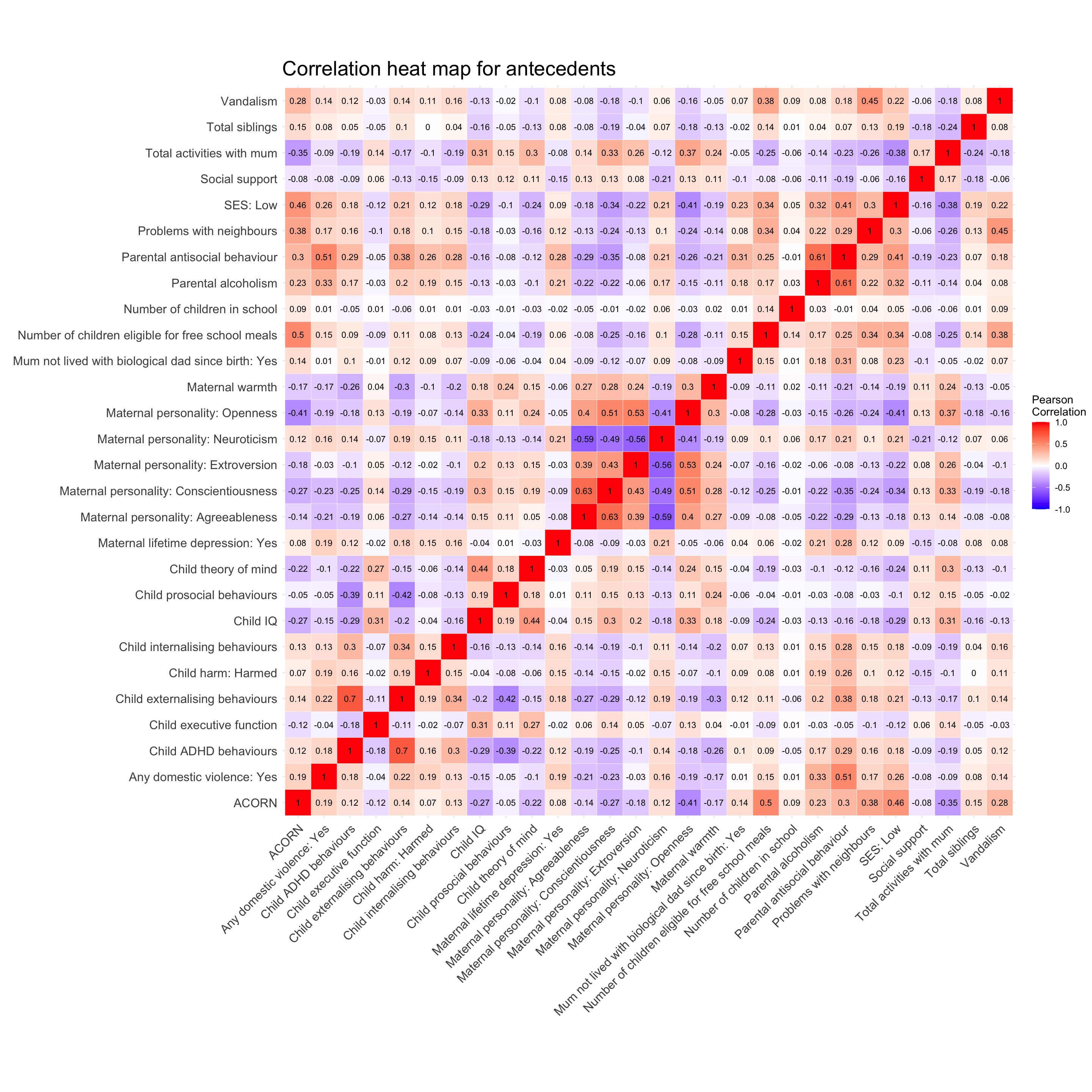

# ggsave(
#   "antecedent_correlation_heat_map.png",
#   plot = correlation_heat_map,
#   device = "png",
#   path = paste0(graph_save_data_path, "antecedents/analysis_interpretation"),
#   width = 15,
#   height = 15
# )

Posterior sensitivity analysis

The below few chunks are used to run the same analysis again in a reduced sample (only individuals who had a posterior probability of above 0.8 in all classes).

IMPORTANT: We created the current Rmd script to be able to use the same script to run the same analysis again in a reduced sample as a sensitivity analysis (only individuals who had a posterior probability of above 0.8 in all classes). When the variable “posterior.cut” is set to TRUE the following code will run for the data set that has those probability<0.8 dropped.

posterior.cut = FALSE

if(posterior.cut == TRUE){

# create new variable only with those who have a probability higher than 0.8 for each class
dat <- dat %>%
  mutate(class_renamed_cut =
           factor(
             case_when(
             prob2 > 0.8 & class_renamed == "Increasing" ~ "Increasing",
             prob3 > 0.8 & class_renamed == "Decreasing" ~ "Decreasing",
             prob1 > 0.8 & class_renamed == "Low stable" ~ "Low stable"
           ), 
           ordered = FALSE))

library(nnet)
# check the biggest group in the class to be the reference group
table(dat$class_renamed_cut)

# relevel class_factor
dat <- dat %>% 
  mutate(
    class_reordered_cut =
      relevel(
        class_renamed_cut,
        ref = "Low stable",
        first = TRUE, #levels in ref come first
        collapse = "+", #String used when constructing names for combined factor levels
        xlevels = TRUE #levels maintained even if not actually occurring
        
      )
  )
# check
table(dat$class_reordered_cut)

# create new data set with only these individuals
dat_prob_cut_out <- dat %>% filter(is.na(class_reordered_cut))
dat <- dat %>% filter(!is.na(class_reordered_cut))

# check
freq(dat$class_reordered)
}

Statistics for posterior probability sensitivity analyses:

Low stable: Dropped 42 people. Average probability = 0.66, minimum probability = 0.48.
Increasing: Dropped 24 people. Average probability = 0.64, minimum probability = 0.49.
Decreasing: Dropped 25 people. Average probability = 0.63, minimum probability = 0.51.

Posterior sensitivity N = 2141

if(posterior.cut == TRUE){
low.stable.cut.stats <- dat_prob_cut_out %>%
  filter(class_reordered == "Low stable") %>%
  descr(prob1)

increasing.cut.stats <- dat_prob_cut_out %>%
  filter(class_reordered == "Increasing") %>%
  descr(prob2)

decreasing.cut.stats <- dat_prob_cut_out %>%
  filter(class_reordered == "Decreasing") %>%
  descr(prob3)

low.stable.cut.stats
increasing.cut.stats
decreasing.cut.stats
}

Antecedent analysis

The following variables were dropped for the analyses: multinom.class_size_average_05, multinom.resident_moves_05, multinom.temp_negative_affect_05, multinom.temp_impulsivity_05, multinom.temp_approach_05, multinom.temp_sluggishness_05, multinom.temp_wariness_05, multinom.temp_undercontrolled_05, multinom.temp_inhibited_05, multinom.temp_shy_05.

Analysis plan

Individual antecedent regressions: single regressions are computed for each variable (class ~ variable). This is done through a loop. Relative Risk Ratios (RRR) and their confidence intervals are calculated. Statistics for all variables are combined and RRR (95% CI) are plotted for the Increasing and Decreasing class.
Full model: All variables that significantly predict class membership are controlled for. E.g. (class ~ social_variable_1 + home_variable_2 + neuro_variable_3 + emo_variable_4). RRR (95% CI) are calculated. Z scores for continuous variables are used. No multiple testing correction is applied at this step.

All regressions are first computed in STATA - multinomial regression with clustering is not currently doable in R. The coefficients are then imported into R to be interpreted. The RRR coefficient indicates the likelihood of having higher values on the variable of interest, for those following either the increasing and decreasing class compared to the low stable.

Binary variables: SES (middle/high vs low), Child harm (No harm vs possible/definite), any domestic violence (Yes/No), maternal lifetime depression (Yes/No). ACORN (1-5) and maternal warmth (1-6) have been recoded to be continuous variables.

STATA file preparation

Create z scores for all continuous variables

# create a scaled version of the continuous variables - z scores for all variables
scaled_continuous_data <- as.data.frame(scale(dat[antecedent.independent.continuous], center = TRUE, scale = TRUE))

# rename variables to show that they are z scores 
colnames(scaled_continuous_data) <- paste0("z_score.", colnames(scaled_continuous_data))

# combine the scaled data to the main dataset 
dat <- cbind(dat, scaled_continuous_data)

Create STATA file

data.mlogit <- dat %>% # need to rename for stata format
  select(id,
         familyid,
         sex,
         classreordered = class_reordered,
         ses = SES_binary_releveled,
         acorn = z_score.acorn_continuous_05,
         vandalism = z_score.vandalism_05,
         probneighbours = z_score.problems_neighbours_05,
         numberchildschool = z_score.number_children_school_05,
         meals = z_score.number_children_school_free_meals_05,
         harm = child_harm_recoded_05,
         siblings = z_score.total_siblings_05,
         socialsupport = z_score.total_social_support_05,
         activities = z_score.total_activities_with_mum_05,
         biodad = mum_notlived_biodad_sincebirth_05,
         domesticviolence = any_domestic_violence_05,
         maternalwarmth = z_score.maternal_warmth_continuous_05,
         maternaldepression = maternal_depression_lifetime_05,
         openness = z_score.maternal_personality_openness_05,
         conscientiousness = z_score.maternal_personality_conscientiousness_05,
         extroversion = z_score.maternal_personality_extroversion_05,
         agreeableness = z_score.maternal_personality_agreeableness_05,
         neuroticism = z_score.maternal_personality_neuroticism_05,
         antisocial = z_score.antisocial_behaviour_parent_05,
         alcohol = z_score.alcoholism_parent_05,
         iq = z_score.IQ_05,
         execfunction = z_score.executive_function_05,
         theoryofmind = z_score.theory_of_mind_05,
         externalising = z_score.externalising_combined_05,
         internalising = z_score.internalising_combined_excl_sis_05,
         adhd = z_score.ADHD_combined_05,
         prosocial = z_score.prosocial_behaviours_combined_05)

Write data files for STATA to be used in multinomial regression. We have saved two different files depending on if we’re doing the sensitivity analysis (reduced sample) or not.

library(foreign)
if(posterior.cut == FALSE){
  write.dta(data.mlogit, "/Users/katiethompson/Documents/PhD/LISS-DTP_Louise_and_Tim/Social isolation trajectories_Paper 1/data_analysis/data_full/data_raw/multinom.reg.stata.dta")
}

if(posterior.cut == TRUE){
  write.dta(data.mlogit, "/Users/katiethompson/Documents/PhD/LISS-DTP_Louise_and_Tim/Social isolation trajectories_Paper 1/data_analysis/data_full/data_raw/multinom.reg.stata.POSTERIOR.dta")
}

STATA multinomial regressions

The mlogit code was run in STATA to calculate RRR, CI and pvalues for all antecedents entered into a single multinomial regression model. If you would like to run this in STATA, you can open the STATA file “antecedent_multinomial_regression.do” or “antecedent_multinomial_regression_POSTERIOR.do” from the Github home page. The output from the STATA file is saved as a txt file containing all the information from the regressions.

Three models were run in STATA:

Individual regressions. Each antecedent was regressed on class membership.
Significant from univariate model. This was NOT taken forward into analyses - only the individual and full model to avoid a stepwise approach
All model. This includes all antecedents in one model predicting class membership.

// read in file
use "multinom.reg.stata.dta"

// create list of outcome variables
local outcomes "ses acorn vandalism probneighbours numberchildschool meals harm siblings socialsupport activities biodad domesticviolence maternalwarmth maternaldepression openness conscientiousness extroversion agreeableness neuroticism antisocial alcohol iq execfunction theoryofmind externalising internalising adhd prosocial"

// loop for multinomial regression clustered by familyid
foreach var of varlist `outcomes' {
mlogit classreordered `var' sex, cluster(familyid)

estimates store results_`var'
}

// install package estout
// ssc install estout

// save results, dropping estimates we don't need and saving the RRR and upper and lower CI for each variable 
estout results_* using multinomial_results_si.txt, drop(sex) cells(b(fmt(2)) ci_l(fmt(2)) ci_u(fmt(2)) p(fmt(8))) eform replace

// all model - predictors that are significant from UNIVARIATE models
mlogit classreordered ses acorn probneighbours meals harm siblings socialsupport activities biodad domesticviolence maternalwarmth maternaldepression openness conscientiousness extroversion agreeableness neuroticism antisocial alcohol iq execfunction theoryofmind externalising internalising adhd prosocial sex, cluster(familyid)
estimates store allmodelsiguni 
estout allmodelsiguni using multinomial_results_si.allmodel.SIGUNI.txt, drop(sex) cells(b(fmt(2)) ci_l(fmt(2)) ci_u(fmt(2)) p(fmt(8))) eform replace

// all model - all predictors in one model
mlogit classreordered ses acorn vandalism probneighbours numberchildschool meals harm siblings socialsupport activities biodad domesticviolence maternalwarmth maternaldepression openness conscientiousness extroversion agreeableness neuroticism antisocial alcohol iq execfunction theoryofmind externalising internalising adhd prosocial sex, cluster(familyid)
estimates store allmodel 
estout allmodel using multinomial_results_si.allmodel.txt, drop(sex) cells(b(fmt(2)) ci_l(fmt(2)) ci_u(fmt(2)) p(fmt(8))) eform replace

Th next bit of code reades the files and moves the txt files to the right place - once this has been done the code is hashed out.

if(posterior.cut == FALSE){
# move txt file to data file 
# file.move(paste0(stata_data_path, "multinomial_results_si.txt"), data_path, overwrite = TRUE)
# file.move(paste0(stata_data_path,"multinomial_results_si.allmodel.SIGUNI.txt"), data_path, overwrite = TRUE)
# file.move(paste0(stata_data_path,"multinomial_results_si.allmodel.txt"), data_path, overwrite = TRUE)
  
# individual regressions
dat.stata.individual.raw <- read_tsv(paste0(data_path, "multinomial_results_si.txt")) 
# all model with only univariate sig variables
dat.stata.all.siguni.raw <- read_tsv(paste0(data_path, "multinomial_results_si.allmodel.SIGUNI.txt"))
# all model
dat.stata.all.raw <- read_tsv(paste0(data_path, "multinomial_results_si.allmodel.txt"))
}

if(posterior.cut == TRUE){
# move txt file to data file 
# file.move(paste0(stata_data_path, "multinomial_results_si_POSTERIOR.txt"), data_path, overwrite = TRUE)
# file.move(paste0(stata_data_path,"multinomial_results_si.allmodel.SIGUNI_POSTERIOR.txt"), data_path, overwrite = TRUE)
# file.move(paste0(stata_data_path,"multinomial_results_si.allmodel_POSTERIOR.txt"), data_path, overwrite = TRUE)

# individual regressions
dat.stata.individual.raw <- read_tsv(paste0(data_path, "multinomial_results_si_POSTERIOR.txt")) 
# all model with only univariate sig variables
dat.stata.all.siguni.raw <- read_tsv(paste0(data_path, "multinomial_results_si.allmodel.SIGUNI_POSTERIOR.txt"))
# all model
dat.stata.all.raw <- read_tsv(paste0(data_path, "multinomial_results_si.allmodel_POSTERIOR.txt"))
}

Reformat STATA output

Layout from the STATA output file:

b/min95/max95/p

We now rearrange this file to create the antecedent multinomial tables needed for the manuscript.

Univariate regressions

dat.stata.individual <- dat.stata.individual.raw[c(120:231,237:348),-c(1)] %>%
  `colnames<-`(name.list) %>%
  mutate(Class =
    case_when(
    row_number() < 113 ~ "Increasing",
    row_number() > 112 ~ "Decreasing")) %>%
  mutate(Variable = 
           rep(c("RRR", "RRR.conf.low", "RRR.conf.high", "p.value"), 56)) %>%
  gather(key, value, `SES: Low`:`Child prosocial behaviours`, factor_key = TRUE) %>%
  drop_na() %>%
  spread(Variable, value) %>%
  dplyr::rename(Variable = key) %>%
  mutate(
    Significance = 
      if_else(
        p.value < 0.05, 
        1,
        0
      ) %>%
    recode_factor(
        "0" = "Non-significant",
        "1" = "Significant")) %>%
  mutate(
    block = 
      case_when(row_number() < 7 ~ "Social domain",
                row_number() < 14 ~ "Home domain",
                row_number() < 22 ~ "Parent domain",
                row_number() < 25 ~ "Neuro domain",
                row_number() < 29 ~ "Emo/behave domain",
                row_number() < 35 ~ "Social domain",
                row_number() < 42 ~ "Home domain",
                row_number() < 50 ~ "Parent domain",
                row_number() < 53 ~ "Neuro domain",
                row_number() > 52 ~ "Emo/behave domain")) %>%
  transmute(Class = Class,
            Variable = Variable,
            RRR = as.numeric(RRR),
            RRR.conf.low = as.numeric(RRR.conf.low),
            RRR.conf.high = as.numeric(RRR.conf.high),
            p.value = as.numeric(p.value),
            Significance = Significance,
            Domain = block)

Table

univariate.reg.table <- paper.table(dat.stata.individual)
univariate.reg.table

Class	Variable	RRR	95% CI low	95% CI high	p value	Domain
Decreasing	SES: Low	1.95	1.32	2.90	0.00	Social domain
Decreasing	ACORN	1.27	1.04	1.55	0.02	Social domain
Decreasing	Vandalism	1.17	0.98	1.39	0.08	Social domain
Decreasing	Problems with neighbours	1.22	1.04	1.44	0.01	Social domain
Decreasing	Number of children in school	1.18	0.95	1.47	0.14	Social domain
Decreasing	Number of children eligible for free school meals	1.37	1.16	1.62	0.00	Social domain
Increasing	SES: Low	2.56	1.68	3.91	0.00	Social domain
Increasing	ACORN	1.27	1.00	1.60	0.05	Social domain
Increasing	Vandalism	1.17	0.96	1.43	0.13	Social domain
Increasing	Problems with neighbours	1.32	1.12	1.54	0.00	Social domain
Increasing	Number of children in school	1.03	0.80	1.32	0.84	Social domain
Increasing	Number of children eligible for free school meals	1.16	0.95	1.42	0.14	Social domain
Decreasing	Child harm: Harmed	2.53	1.63	3.93	0.00	Home domain
Decreasing	Total siblings	1.24	1.05	1.47	0.01	Home domain
Decreasing	Social support	0.77	0.63	0.95	0.01	Home domain
Decreasing	Total activities with mum	0.70	0.57	0.85	0.00	Home domain
Decreasing	Mum not lived with biological dad since birth: Yes	1.84	0.91	3.70	0.09	Home domain
Decreasing	Any domestic violence: Yes	1.82	1.22	2.71	0.00	Home domain
Decreasing	Maternal warmth	0.66	0.55	0.80	0.00	Home domain
Increasing	Child harm: Harmed	1.66	0.98	2.81	0.06	Home domain
Increasing	Total siblings	1.04	0.82	1.31	0.75	Home domain
Increasing	Social support	0.77	0.63	0.94	0.01	Home domain
Increasing	Total activities with mum	0.65	0.54	0.78	0.00	Home domain
Increasing	Mum not lived with biological dad since birth: Yes	2.25	1.15	4.42	0.02	Home domain
Increasing	Any domestic violence: Yes	1.42	0.93	2.18	0.10	Home domain
Increasing	Maternal warmth	0.64	0.52	0.80	0.00	Home domain
Decreasing	Maternal lifetime depression: Yes	1.88	1.27	2.78	0.00	Parent domain
Decreasing	Maternal personality: Openness	0.80	0.65	0.97	0.03	Parent domain
Decreasing	Maternal personality: Conscientiousness	0.58	0.49	0.70	0.00	Parent domain
Decreasing	Maternal personality: Extroversion	0.77	0.64	0.93	0.01	Parent domain
Decreasing	Maternal personality: Agreeableness	0.66	0.54	0.81	0.00	Parent domain
Decreasing	Maternal personality: Neuroticism	1.45	1.20	1.75	0.00	Parent domain
Decreasing	Parental antisocial behaviour	1.63	1.40	1.91	0.00	Parent domain
Decreasing	Parental alcoholism	1.35	1.17	1.57	0.00	Parent domain
Increasing	Maternal lifetime depression: Yes	1.25	0.82	1.92	0.30	Parent domain
Increasing	Maternal personality: Openness	0.66	0.53	0.81	0.00	Parent domain
Increasing	Maternal personality: Conscientiousness	0.65	0.54	0.79	0.00	Parent domain
Increasing	Maternal personality: Extroversion	0.72	0.59	0.88	0.00	Parent domain
Increasing	Maternal personality: Agreeableness	0.74	0.61	0.89	0.00	Parent domain
Increasing	Maternal personality: Neuroticism	1.33	1.09	1.62	0.00	Parent domain
Increasing	Parental antisocial behaviour	1.42	1.18	1.71	0.00	Parent domain
Increasing	Parental alcoholism	1.15	0.98	1.34	0.08	Parent domain
Decreasing	Child IQ	0.56	0.46	0.69	0.00	Neuro domain
Decreasing	Child executive function	0.66	0.55	0.79	0.00	Neuro domain
Decreasing	Child theory of mind	0.61	0.49	0.77	0.00	Neuro domain
Increasing	Child IQ	0.64	0.51	0.79	0.00	Neuro domain
Increasing	Child executive function	0.88	0.73	1.06	0.19	Neuro domain
Increasing	Child theory of mind	0.65	0.52	0.81	0.00	Neuro domain
Decreasing	Child externalising behaviours	2.47	2.11	2.89	0.00	Emo/behave domain
Decreasing	Child internalising behaviours	3.37	2.79	4.08	0.00	Emo/behave domain
Decreasing	Child ADHD behaviours	2.85	2.38	3.41	0.00	Emo/behave domain
Decreasing	Child prosocial behaviours	0.42	0.34	0.51	0.00	Emo/behave domain
Increasing	Child externalising behaviours	2.06	1.77	2.39	0.00	Emo/behave domain
Increasing	Child internalising behaviours	1.66	1.38	1.99	0.00	Emo/behave domain
Increasing	Child ADHD behaviours	2.39	2.02	2.82	0.00	Emo/behave domain
Increasing	Child prosocial behaviours	0.64	0.53	0.78	0.00	Emo/behave domain

Bind z score trasformed values to order the graph according to block of variables

individual.home <- order.variables(data = dat.stata.individual, domain = "Home domain")
individual.social <- order.variables(data = dat.stata.individual, domain = "Social domain")
individual.parent <- order.variables(data = dat.stata.individual, domain = "Parent domain")
individual.neuro <- order.variables(data = dat.stata.individual, domain = "Neuro domain")
individual.emo <- order.variables(data = dat.stata.individual, domain = "Emo/behave domain")

# join all
dat.stata.individual.ordered <- rbind(
  individual.social,
  individual.home,
  individual.parent,
  individual.neuro,
  individual.emo
)

Plot for univariate regressions

stata.plot.individual <- ggplot(
  dat.stata.individual.ordered, 
  aes(x = Variable,
      y = RRR,
      ymin = RRR.conf.low,
      ymax = RRR.conf.high,)
  ) +
  scale_fill_manual(values = "black") +
  scale_color_manual(values = "black") +
  scale_shape_manual(values = c(19)) +
  geom_pointrange(position = position_dodge(width = 0.7), 
                  show.legend = FALSE, 
                  size = 0.5) +
 facet_grid(Domain ~ Class, drop = TRUE, scales = "free_y", space = "free") +
  labs(y = "RRR (95% CI)",
       x = "names",
       shape = "") +
  theme.antecedent +
  geom_hline(linetype = "dashed", yintercept = 1) +
 scale_y_continuous(trans = scales::log10_trans(), breaks=c(0.4,0.6,0.8, 1, 1.5, 2, 2.5, 3, 3.5, 4)) +
  coord_flip()

stata.plot.individual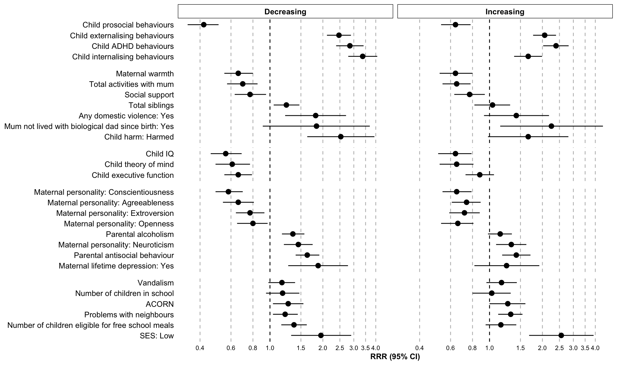

Multivariate model: all variables included

dat.stata.all <- dat.stata.all.raw[c(120:231,237:348),] %>%
  mutate(Class =
    case_when(
    row_number() < 113 ~ "Increasing",
    row_number() > 112 ~ "Decreasing")) %>%
  mutate(key = 
           rep(c("RRR", "RRR.conf.low", "RRR.conf.high", "p.value"), 56)) %>%
  mutate(Variable =
    case_when(row_number() < 5  ~ "SES: Low",
              row_number() < 9  ~ "ACORN",
              row_number() < 13 ~ "Vandalism",
              row_number() < 17 ~ "Problems with neighbours",
              row_number() < 21 ~ "Number of children in school",
              row_number() < 25 ~ "Number of children eligible for free school meals",
              row_number() < 29 ~ "Child harm: Harmed",
              row_number() < 33 ~ "Total siblings",
              row_number() < 37 ~ "Social support",
              row_number() < 41 ~ "Total activities with mum",
              row_number() < 45 ~ "Mum not lived with biological dad since birth: Yes",
              row_number() < 49 ~ "Any domestic violence: Yes" ,
              row_number() < 53 ~ "Maternal warmth",
              row_number() < 57 ~ "Maternal lifetime depression: Yes",
              row_number() < 61 ~ "Maternal personality: Openness",
              row_number() < 65 ~ "Maternal personality: Conscientiousness",
              row_number() < 69 ~ "Maternal personality: Extroversion",
              row_number() < 73 ~ "Maternal personality: Agreeableness",
              row_number() < 77 ~ "Maternal personality: Neuroticism",
              row_number() < 81 ~ "Parental antisocial behaviour",
              row_number() < 85 ~ "Parental alcoholism",
              row_number() < 89 ~ "Child IQ",
              row_number() < 93 ~ "Child executive function",
              row_number() < 97 ~ "Child theory of mind",
              row_number() < 101 ~ "Child externalising behaviours" ,
              row_number() < 105 ~ "Child internalising behaviours",
              row_number() < 109 ~ "Child ADHD behaviours",
              row_number() < 113 ~ "Child prosocial behaviours",
              row_number() < 117  ~ "SES: Low",
              row_number() < 121  ~ "ACORN",
              row_number() < 125 ~ "Vandalism",
              row_number() < 129 ~ "Problems with neighbours",
              row_number() < 133 ~ "Number of children in school",
              row_number() < 137 ~ "Number of children eligible for free school meals",
              row_number() < 141 ~ "Child harm: Harmed",
              row_number() < 145 ~ "Total siblings",
              row_number() < 149 ~ "Social support",
              row_number() < 153 ~ "Total activities with mum",
              row_number() < 157 ~ "Mum not lived with biological dad since birth: Yes",
              row_number() < 161 ~ "Any domestic violence: Yes" ,
              row_number() < 165 ~ "Maternal warmth",
              row_number() < 169 ~ "Maternal lifetime depression: Yes",
              row_number() < 173 ~ "Maternal personality: Openness",
              row_number() < 177 ~ "Maternal personality: Conscientiousness",
              row_number() < 181 ~ "Maternal personality: Extroversion",
              row_number() < 185 ~ "Maternal personality: Agreeableness",
              row_number() < 189 ~ "Maternal personality: Neuroticism",
              row_number() < 193 ~ "Parental antisocial behaviour",
              row_number() < 197 ~ "Parental alcoholism",
              row_number() < 201 ~ "Child IQ",
              row_number() < 205 ~ "Child executive function",
              row_number() < 209 ~ "Child theory of mind",
              row_number() < 213 ~ "Child externalising behaviours" ,
              row_number() < 217 ~ "Child internalising behaviours",
              row_number() < 221 ~ "Child ADHD behaviours",
              row_number() > 220 ~ "Child prosocial behaviours")) %>%
  select(-X1) %>%
  mutate(
    block = case_when(
              row_number() < 25  ~ "Social domain",
              row_number() < 53 ~ "Home domain",
              row_number() < 85 ~ "Parent domain",
              row_number() < 97 ~ "Neuro domain",
              row_number() < 113 ~ "Emo/behave domain",
              row_number() < 137 ~ "Social domain",
              row_number() < 165 ~ "Home domain",
              row_number() < 197 ~ "Parent domain",
              row_number() < 209 ~ "Neuro domain",
              row_number() > 208 ~ "Emo/behave domain")) %>%
  spread(key, allmodel) %>%
  mutate(
    Significance = 
      if_else(
        p.value < 0.05, 
        1,
        0
      ) %>%
    recode_factor(
        "0" = "Non-significant",
        "1" = "Significant")) %>%
  transmute(Class = Class,
            Variable = Variable,
            RRR = as.numeric(RRR),
            RRR.conf.low = as.numeric(RRR.conf.low),
            RRR.conf.high = as.numeric(RRR.conf.high),
            p.value = as.numeric(p.value),
            Significance = Significance,
            Domain = block)

Table

paper.table.all.variables <- paper.table(dat.stata.all)
paper.table.all.variables

Class	Variable	RRR	95% CI low	95% CI high	p value	Domain
Decreasing	ACORN	0.91	0.61	1.35	0.64	Social domain
Decreasing	Number of children eligible for free school meals	1.06	0.73	1.54	0.77	Social domain
Decreasing	Number of children in school	1.43	1.07	1.93	0.02	Social domain
Decreasing	Problems with neighbours	0.84	0.59	1.19	0.32	Social domain
Decreasing	SES: Low	1.00	0.48	2.12	0.99	Social domain
Decreasing	Vandalism	0.88	0.63	1.23	0.46	Social domain
Increasing	ACORN	0.94	0.67	1.32	0.71	Social domain
Increasing	Number of children eligible for free school meals	1.02	0.73	1.42	0.91	Social domain
Increasing	Number of children in school	1.07	0.81	1.43	0.62	Social domain
Increasing	Problems with neighbours	1.17	0.89	1.55	0.25	Social domain
Increasing	SES: Low	1.48	0.77	2.83	0.24	Social domain
Increasing	Vandalism	0.80	0.58	1.10	0.17	Social domain
Decreasing	Any domestic violence: Yes	0.93	0.49	1.79	0.84	Home domain
Decreasing	Child harm: Harmed	1.14	0.56	2.33	0.71	Home domain
Decreasing	Maternal warmth	1.06	0.81	1.37	0.68	Home domain
Decreasing	Mum not lived with biological dad since birth: Yes	0.89	0.34	2.32	0.81	Home domain
Decreasing	Social support	0.87	0.64	1.18	0.37	Home domain
Decreasing	Total activities with mum	1.04	0.76	1.43	0.79	Home domain
Decreasing	Total siblings	1.15	0.91	1.45	0.25	Home domain
Increasing	Any domestic violence: Yes	0.75	0.41	1.38	0.36	Home domain
Increasing	Child harm: Harmed	1.19	0.57	2.48	0.65	Home domain
Increasing	Maternal warmth	1.00	0.77	1.30	1.00	Home domain
Increasing	Mum not lived with biological dad since birth: Yes	1.10	0.42	2.87	0.85	Home domain
Increasing	Social support	0.92	0.72	1.18	0.53	Home domain
Increasing	Total activities with mum	0.79	0.60	1.03	0.08	Home domain
Increasing	Total siblings	0.82	0.61	1.11	0.21	Home domain
Decreasing	Maternal lifetime depression: Yes	1.08	0.58	1.99	0.81	Parent domain
Decreasing	Maternal personality: Agreeableness	0.97	0.64	1.46	0.88	Parent domain
Decreasing	Maternal personality: Conscientiousness	0.85	0.60	1.20	0.35	Parent domain
Decreasing	Maternal personality: Extroversion	0.84	0.58	1.22	0.36	Parent domain
Decreasing	Maternal personality: Neuroticism	1.01	0.65	1.57	0.95	Parent domain
Decreasing	Maternal personality: Openness	1.67	1.12	2.50	0.01	Parent domain
Decreasing	Parental alcoholism	1.09	0.80	1.50	0.57	Parent domain
Decreasing	Parental antisocial behaviour	0.93	0.63	1.36	0.69	Parent domain
Increasing	Maternal lifetime depression: Yes	1.12	0.62	2.02	0.70	Parent domain
Increasing	Maternal personality: Agreeableness	0.93	0.67	1.28	0.65	Parent domain
Increasing	Maternal personality: Conscientiousness	1.00	0.69	1.43	0.98	Parent domain
Increasing	Maternal personality: Extroversion	1.05	0.71	1.56	0.82	Parent domain
Increasing	Maternal personality: Neuroticism	0.93	0.66	1.31	0.69	Parent domain
Increasing	Maternal personality: Openness	0.94	0.60	1.48	0.80	Parent domain
Increasing	Parental alcoholism	0.81	0.63	1.04	0.10	Parent domain
Increasing	Parental antisocial behaviour	0.97	0.66	1.44	0.90	Parent domain
Decreasing	Child executive function	0.79	0.62	1.00	0.05	Neuro domain
Decreasing	Child IQ	0.96	0.71	1.28	0.77	Neuro domain
Decreasing	Child theory of mind	1.02	0.74	1.41	0.90	Neuro domain
Increasing	Child executive function	1.30	1.02	1.66	0.04	Neuro domain
Increasing	Child IQ	1.00	0.75	1.34	1.00	Neuro domain
Increasing	Child theory of mind	0.82	0.63	1.07	0.15	Neuro domain
Decreasing	Child ADHD behaviours	1.78	1.25	2.54	0.00	Emo/behave domain
Decreasing	Child externalising behaviours	1.15	0.79	1.67	0.46	Emo/behave domain
Decreasing	Child internalising behaviours	3.02	2.29	3.97	0.00	Emo/behave domain
Decreasing	Child prosocial behaviours	0.59	0.43	0.81	0.00	Emo/behave domain
Increasing	Child ADHD behaviours	1.90	1.40	2.57	0.00	Emo/behave domain
Increasing	Child externalising behaviours	1.30	0.94	1.78	0.11	Emo/behave domain
Increasing	Child internalising behaviours	1.22	0.95	1.56	0.12	Emo/behave domain
Increasing	Child prosocial behaviours	1.01	0.77	1.33	0.95	Emo/behave domain

dat.stata.all.plot <- dat.stata.all %>% 
  filter(Significance == "Significant",
         Variable != "Child executive function")

individual.sig.social.plot <- order.variables(data = dat.stata.all.plot, domain = "Social domain")
individual.sig.parent.plot <- order.variables(data = dat.stata.all.plot, domain = "Parent domain")
individual.sig.emo.plot <- order.variables(data = dat.stata.all.plot, domain = "Emo/behave domain")

# join all
dat.stata.all.plot.ordered <- rbind(
  individual.sig.social.plot,
  individual.sig.parent.plot,
  individual.sig.emo.plot
)

Plot of significant variables from the multivariate analysis:

stata.plot.all_model <- ggplot(
  dat.stata.all.plot.ordered, 
  aes(x = Variable,
      y = RRR,
      ymin = RRR.conf.low,
      ymax = RRR.conf.high,
      color = Class)
  ) +
  scale_fill_manual(values = c("black", "black")) +
  scale_color_manual(values = c("black", "black")) +
  scale_shape_manual(values = c(19)) +
  geom_pointrange(aes(shape = Significance), position = position_dodge(width = 0.7)) +
  facet_grid(Domain ~ Class, drop = TRUE, scales = "free_y", space = "free") +
  labs(y = "RRR (95% CI)",
       x = "names",
       title = "Association between antecedents and social isolation trajectories",
       subtitle = paste("N(Total) = ", length(dat$sex),
                        "; N(Increasing) = ", sum(!is.na(dat$class_renamed[dat$class_renamed=="Increasing"])),
                        "; N(Decreasing) = ", sum(!is.na(dat$class_renamed[dat$class_renamed=="Decreasing"])), sep = ""),
       color = "",
       shape = "") +
  theme.antecedent +
  theme(legend.position = "none") +
  geom_hline(linetype = "dashed", yintercept = 1) +
 scale_y_continuous(trans = scales::log10_trans(), breaks=c(0.5, 0.6,0.8, 1, 1.5, 2, 2.5, 3, 4)) +
  coord_flip()

stata.plot.all_model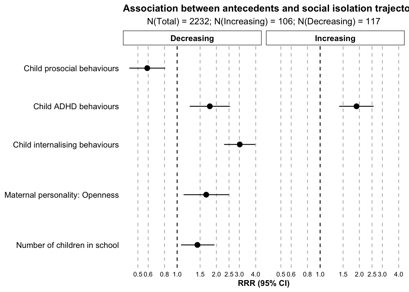

Work by Katherine N Thompson

katherine.n.thompson@kcl.ac.uk

Associations between social isolation trajectories and antecedents

Functions

Test for multicollinearity

Posterior sensitivity analysis

Antecedent analysis

STATA file preparation

STATA multinomial regressions

Reformat STATA output

Univariate regressions

Table

Plot for univariate regressions

Multivariate model: all variables included

Table