Preliminary descriptives for social isolation in E-Risk
This page dispays preliminary descriptive statistics for social isolation variables in E-Risk. The contents are listed on the left hand side of the page. Social isolation was measured using items from the Children’s Behaviour Checklist (CBCL), responses were scored 0 (not true), 1 (somewhat true) and 2 (often true) were summed to make a total score and then were averaged from both parents and teachers:
- “complains of loneliness”
- “doesn’t get along with other children [pupils]”
- “feels or complains that no-one loves him/her”
- “would rather be alone than with others”
- “not liked by other children [pupils]”
- “withdrawn, doesn’t get involved with others”
Missingness descriptives
Visits were conducted when the children were aged 5 (100% participation), 7 (98%), 10 (96%), 12 (96%), and 18 years (93%). Rates of missingness for social isolation items is reported below. First, the number of time points missing per person is reported, then social isolation item frequencies are displayed for each age.
Groups for participants missing 2 or 3 time points
To check that data is missing at random (MAR), we created two variables that indicate group membershop based on missingness. The first variable split those that were missing three time points (N=18) into one group, and everyone else in another group. The second variable split those that were missing two time points (N=46) into one group (exluding those missing three time points), and those missing 1 or zero into the other group. We then tested for differences in social isolation, SES, IQ, internalising behaviours, and extermalising behaviours at age 5, dependednt on the two mimssingness group variables created.
# group with 18 missing 3 time points vs everyone else
dat <- dat %>%
  mutate(
    missing_3_time_points =
      if_else(
        na.per.person.si > 2,
        1,
        0) %>%
      recode_factor(
        "0" = "No",
        "1" = "Yes"
      )
  )

# create group of just 18 who have 3 missing time points
dat.18 <- filter(dat, missing_3_time_points == "Yes")

# excluding the 18 missing 3 time points, those with 2 missing time points vs every one else
dat.missing.3time <- filter(dat,
                      na.per.person.si != 3)

dat.missing.3time <- dat.missing.3time %>%
  mutate(
    missing_2_time_points =
      if_else(
        na.per.person.si > 1 & na.per.person.si < 3,
        1,
        0) %>%
      recode_factor(
        "0" = "No",
        "1" = "Yes"
      )
)Missingness differences at age 18
We found no differences between those who did and did not take part at age 18 in terms of socioeconomic status (SES) assessed when the cohort was initially defined (χ2 = 0.86, p = 0.65), age-5 IQ scores (t = 0.98, p = 0.33), or age-5 emotional or behavioural problems (t = 0.40, p = 0.69 and t = 0.41, p = 0.68, respectively). There were 2066 complete responses at age 18 (92.56% retention).
# check the freq
employment.freq <- freq(dat$not_in_employment_education_18,
     cumul = FALSE)

# create data set for those who did and did not take part at age 18
## 166 participants
dat_not_age_18 <- dat %>%
  filter(is.na(not_in_employment_education_18))
## 2066 participants
dat_age_18 <- dat %>%
  filter(!is.na(not_in_employment_education_18))

# create variable in original data set based on cut off
dat <- dat %>%
  mutate(
    took_part_at_18 =
      if_else(
        !is.na(not_in_employment_education_18),
        1,
        0) %>%
      recode_factor(
        "0" = "No",
        "1" = "Yes"
      )
  )

# check
# table(dat$took_part_at_18)

# Social isolation - t-test - nonsig
ttest_SI_age18 <- t.test(
  isolation_combined_05 ~ took_part_at_18,
  data = dat,
  alternative = "two.sided",
  conf.level = 0.95)

# IQ - t-test - nonsig
ttest_IQ_age18 <- t.test(
  IQ_05 ~ took_part_at_18,
  data = dat,
  alternative = "two.sided",
  conf.level = 0.95)

# externalising - t-test - nonsig
ttest_ext_age18 <- t.test(
  externalising_combined_05 ~ took_part_at_18,
  data = dat,
  alternative = "two.sided",
  conf.level = 0.95)

# internalising - t-test - nonsig
ttest_int_age18 <- t.test(
  internalising_combined_excl_sis_05 ~ took_part_at_18,
  data = dat,
  alternative = "two.sided",
  conf.level = 0.95)

# SES - chi square
chisq_SES_age18 <- chisq.test(dat$SES,
                              dat$took_part_at_18) # nonsig
Means across all time points
Below are the mean social isolation scores plotted for each time point. Underneath are the descriptives for social isolation stratified by combined report (mother and teacher), mother report, and teacher report.
#summarize the data fir the plot
dat_summary.isolation <- summarySE(dat_long,
                            measurevar = "social_isolation",
                            groupvars = c("time_point"),
                            na.rm=TRUE)
#create plot
diff.plot <- ggplot(dat_summary.isolation,
       aes(x = time_point,
           y = social_isolation,
           group = 1)) +
    geom_errorbar(aes(ymin = social_isolation - se,
                      ymax = social_isolation + se),
                  colour = "black",
                  width = 0.1) +
    geom_line(colour = "red") +
    geom_point(size = 3,
               shape = 21,
               fill = "white") + # 21 is filled circle
    xlab("Time point") +
    ylab("Social isolation") +
    ggtitle("Average differences in social isolation at time point 5, 7, 10 and 12") +
    expand_limits(y = 0) +
    scale_y_continuous(expand = c(0.1,0.1),
                     limits = c(0,12),
                     breaks = seq(0, 12, 2)) +
  theme_bw()

#create scaled plot
diff.plot.scaled <- diff.plot+
  scale_y_continuous(expand = c(0.1,0.1),
                     limits = c(0,2),
                     breaks = seq(0, 2, 0.25)) +
   ggtitle("Scaled average differences in social isolation at time point 5, 7, 10 and 12")
diff.plot.scaled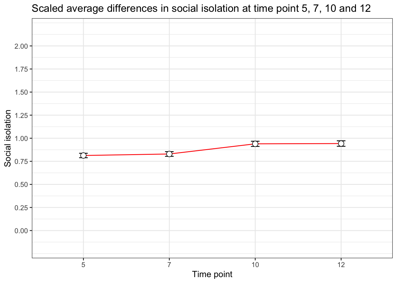
Teacher report
dat %>%
  select(`Age five` = isolation_teacher_05,
         `Age seven` = isolation_teacher_07,
         `Age ten` = isolation_teacher_10,
         `Age twelve` = isolation_teacher_12) %>%
  descr(
      headings = FALSE,
      stats =  c("mean", "sd", "min", "max", "skewness", "kurtosis", "n.valid", "pct.valid"),
style = "rmarkdown") | Age five | Age seven | Age ten | Age twelve | |
|---|---|---|---|---|
| Mean | 0.62 | 0.64 | 0.72 | 0.77 |
| Std.Dev | 1.25 | 1.31 | 1.46 | 1.49 |
| Min | 0.00 | 0.00 | 0.00 | 0.00 |
| Max | 12.00 | 10.00 | 12.00 | 12.00 |
| Skewness | 3.08 | 3.05 | 2.85 | 2.56 |
| Kurtosis | 13.16 | 11.56 | 9.76 | 7.71 |
| N.Valid | 2093.00 | 2026.00 | 1924.00 | 1775.00 |
| Pct.Valid | 93.77 | 90.77 | 86.20 | 79.53 |
Social isolation split by sex
Below are violin plots showing social isolation combined report scores stratified by sex.
Age 5
dat %>%
  ggplot(
    mapping = aes(
    x = sex,
    y = isolation_combined_05,
    fill = sex)) +
  geom_hline(yintercept = 5, linetype = "dashed", color = "gray") +
  geom_hline(yintercept = 10, linetype = "dashed", color = "gray") +
  geom_hline(yintercept = 15, linetype = "dashed", color = "gray") +
  geom_flat_violin(
    position = position_nudge(x = .2, y = 0),
    trim = FALSE,
    alpha = 0.5
    ) +
  geom_point(
    aes(
      y = isolation_combined_05,
      color = sex),
    position = position_jitter(width = .15),
    size = .5,
    alpha = 0.8) +
 stat_summary(fun = mean,
              fun.min = function(x) mean(x)* sd(x),
              fun.max = function(x) mean(x) + sd(x),
              geom = "pointrange"
              ) +
  labs(
    title = "Social isolation in males and females at age 5",
    y = "Social isolation",
    fill = "Sex") +
  theme_personal +
  theme(
    axis.text.y = element_blank()
  ) +
  scale_fill_manual(
    values = palette2,
    breaks = c("Male", "Female")
) +
  scale_alpha(guide = 'none') +
  scale_size(guide = 'none') +
  scale_color_manual(
    values = palette2,
    breaks = c("Male", "Female"),
    guide = "none") +
  coord_flip()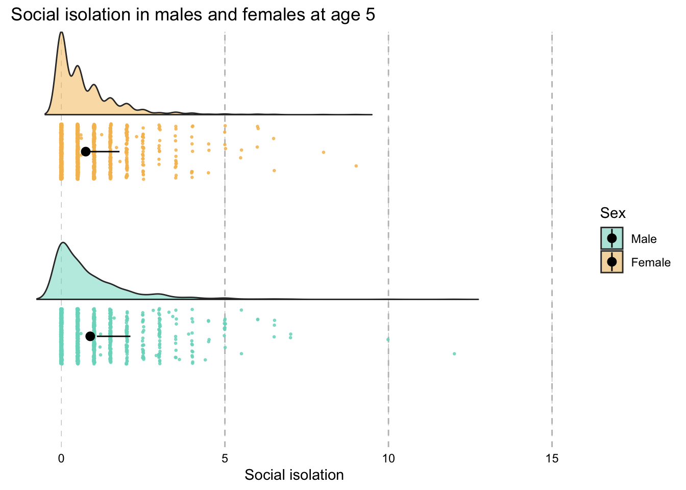
Age 7
dat %>%
  ggplot(
    mapping = aes(
    x = sex,
    y = isolation_combined_07,
    fill = sex)) +
  geom_hline(yintercept = 5, linetype = "dashed", color = "gray") +
  geom_hline(yintercept = 10, linetype = "dashed", color = "gray") +
  geom_hline(yintercept = 15, linetype = "dashed", color = "gray") +
  geom_flat_violin(
    position = position_nudge(x = .2, y = 0),
    trim = FALSE,
    alpha = 0.5
    ) +
  geom_point(
    aes(
      y = isolation_combined_05,
      color = sex),
    position = position_jitter(width = .15),
    size = .5,
    alpha = 0.8) +
 stat_summary(fun = mean,
              fun.min = function(x) mean(x)* sd(x),
              fun.max = function(x) mean(x) + sd(x),
              geom = "pointrange"
              ) +
  labs(
    title = "Social isolation in males and females at age 7",
    y = "Social isolation",
    fill = "Sex") +
  theme_personal +
  theme(
    axis.text.y = element_blank()
  ) +
  scale_fill_manual(
    values = palette2,
    breaks = c("Male", "Female")
) +
  scale_alpha(guide = 'none') +
  scale_size(guide = 'none') +
  scale_color_manual(
    values = palette2,
    breaks = c("Male", "Female"),
    guide = "none") +
  coord_flip()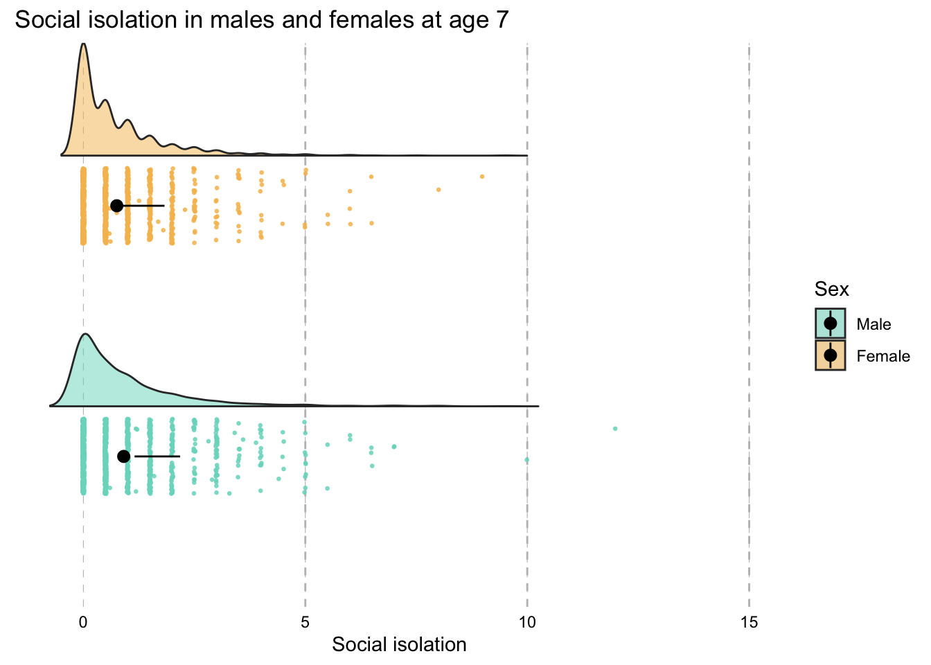
Age 10
dat %>%
  ggplot(
    mapping = aes(
    x = sex,
    y = isolation_combined_10,
    fill = sex)) +
  geom_hline(yintercept = 5, linetype = "dashed", color = "gray") +
  geom_hline(yintercept = 10, linetype = "dashed", color = "gray") +
  geom_hline(yintercept = 15, linetype = "dashed", color = "gray") +
  geom_flat_violin(
    position = position_nudge(x = .2, y = 0),
    trim = FALSE,
    alpha = 0.5
    ) +
  geom_point(
    aes(
      y = isolation_combined_05,
      color = sex),
    position = position_jitter(width = .15),
    size = .5,
    alpha = 0.8) +
 stat_summary(fun = mean,
              fun.min = function(x) mean(x)* sd(x),
              fun.max = function(x) mean(x) + sd(x),
              geom = "pointrange"
              ) +
  labs(
    title = "Social isolation in males and females at age 10",
    y = "Social isolation",
    fill = "Sex") +
  theme_personal +
  theme(
    axis.text.y = element_blank()
  ) +
  scale_fill_manual(
    values = palette2,
    breaks = c("Male", "Female")
) +
  scale_alpha(guide = 'none') +
  scale_size(guide = 'none') +
  scale_color_manual(
    values = palette2,
    breaks = c("Male", "Female"),
    guide = "none") +
  coord_flip()
Age 12
dat %>%
  ggplot(
    mapping = aes(
    x = sex,
    y = isolation_combined_12,
    fill = sex)) +
  geom_hline(yintercept = 5, linetype = "dashed", color = "gray") +
  geom_hline(yintercept = 10, linetype = "dashed", color = "gray") +
  geom_hline(yintercept = 15, linetype = "dashed", color = "gray") +
  geom_flat_violin(
    position = position_nudge(x = .2, y = 0),
    trim = FALSE,
    alpha = 0.5
    ) +
  geom_point(
    aes(
      y = isolation_combined_05,
      color = sex),
    position = position_jitter(width = .15),
    size = .5,
    alpha = 0.8) +
 stat_summary(fun = mean,
              fun.min = function(x) mean(x)* sd(x),
              fun.max = function(x) mean(x) + sd(x),
              geom = "pointrange"
              ) +
  labs(
    title = "Social isolation in males and females at age 12",
    y = "Social isolation",
    fill = "Sex") +
  theme_personal +
  theme(
    axis.text.y = element_blank()
  ) +
  scale_fill_manual(
    values = palette2,
    breaks = c("Male", "Female")
) +
  scale_alpha(guide = 'none') +
  scale_size(guide = 'none') +
  scale_color_manual(
    values = palette2,
    breaks = c("Male", "Female"),
    guide = "none") +
  coord_flip()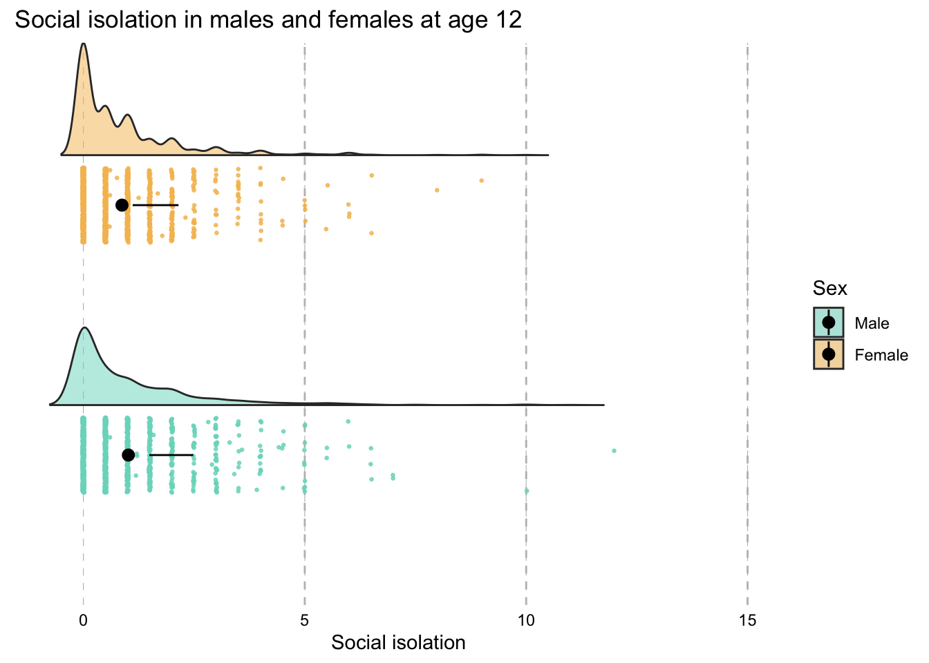
Work by Katherine N Thompson
katherine.n.thompson@kcl.ac.uk
Social isolation at age 5
Social isolation at age five was not significantly different for those missing three time points, compared to everyone else (t =0.713, df=17.245, p=0.485). Mean for group not missing three time points = 0.815, mean for group missing three three time points = 0.611.
Social isolation at age five was not significantly different for those missing two time points, compared to everyone else (t =-0.799, df=46.422, p=0.429). Mean for group not missing two time points = 0.811, mean for group missing two three time points = 0.967.