Associations between social isolation trajectories and outcomes at age 18
This page displays the results from logistic and linear multivariate regressions used to assess how the outcomes at age 18 are associated with social isolation trajectory membership. Outcomes are sorted into domains of “Mental health”, “Physical health”, “Coping and functioning”, and “Employment prospects”.
Functions
To run the following code more clearly, I have created these functions:
- multiple.testing() applies the BH multiple testing correction. You define the data, class, method and number of tests.
- add.significance.variable() add’s a variable to the dataset that labels if a result has a significant p value or not.
- paper.table() creates a table that is formatted correctly for either linear or logitic regression results.
- create.dataset() binds regression results together to form a data set.
- huber.white.cluster.logistic() applies heteroskedasticity-robust standard errors while clustering for familyid for logistic regression
- order.variables() orders the data whereby points in a plot are arranged by OR/Beta and domain.
- reorder_cor_matrix() orders the correlation matrix for the heat map
- huber.white.cluster.linear() applies heteroskedasticity-robust standard errors while clustering for familyid for linear regression
multiple.testing <- function(data, class, method = "BH", n.tests){
  data <- data %>%
    filter(Class == class) %>%
  mutate(
    p.value.adjusted =
           stats::p.adjust(p.value,
                    method = method,
                    n = n.tests)
  ) %>%
  mutate(Significance.adjusted =
           if_else(
            p.value.adjusted < 0.05,
            1,
            0
      ) %>%
        recode_factor(
          `1` = "Significant",
          `0` = "Non-significant")
         )
  return(data)
}

add.significance.variable <- function(data){
  data <- data %>%
    mutate(
    Significance =
      if_else(
        p.value < 0.05,
        1,
        0
      ) %>%
    recode_factor(
        "0" = "Non-significant",
        "1" = "Significant"
      ))
  return(data)
}

paper.table <- function(data, model){
  if (model == "logistic"){
  table <- data %>%
    select(
    Class,
    Variable,
    OR,
    `95% CI low` = OR.conf.low,
    `95% CI high` = OR.conf.high,
    `p value` = p.value,
    Domain,
    -Significance) %>%
  kable(digits = 2)
  return(table)}

  else if (model == "linear"){
    table <- data %>%
    select(
    Class,
    Variable,
    `Beta estimate` = estimate,
    `95% CI low` = conf.low,
    `95% CI high` = conf.high,
    `p value` = p.value,
    Domain,
    -Significance) %>%
  kable(digits = 2)
  return(table)
  }
}

create.dataset <- function(data, model){
  if (model == "logistic"){
  data <- data.table::rbindlist(data) %>%
  dplyr::select(Class,
         Variable,
         OR,
         OR.conf.low,
         OR.conf.high,
         p.value,
         Significance,
         Domain = block)
  return(data)}
  else if (model == "linear"){
  data <- data.table::rbindlist(data) %>%
  dplyr::select(Class,
         Variable,
         estimate,
         robust.std.error,
         conf.low,
         conf.high,
         p.value,
         Significance,
         Domain = block)
  return(data)
  }
}

huber.white.cluster.logistic <- function(regression.outcome){
   outcome.full <- summ(regression.outcome,
                       scale = FALSE,          # standardized regression coefficients
                       confint = TRUE,        # report confidence intervals over standard errors
                       ci.width = 0.95,       # desired confidence interval
                       robust = "HC0",        # heteroskedasticity-robust standard errors instead of conventional SEs
                       cluster = "familyid",  # for clustered standard errors, provide column name of cluster variable
                       exp = TRUE)
   return(outcome.full)
}

order.variables <- function(data, domain, model){
  if (model == "logistic"){
  data <- filter(data, Domain == domain) %>%
    arrange(desc(OR))

  data$Variable <- factor(data$Variable,
                          levels = paste(unique(paste(data$Variable)), sep = ","))
  return(data)}
  else if (model == "linear"){
    data <- filter(data, Domain == domain) %>%
    arrange(desc(estimate))

    data$Variable <- factor(data$Variable,
                          levels = paste(unique(paste(data$Variable)), sep = ","))
  return(data)
  }
}

reorder_cor_matrix <- function(cor_matrix){
 dd <- as.dist((1-cor_matrix)/2) #Use correlation between variables as distance
 hc <- hclust(dd)
 cormat <-cor_matrix[hc$order, hc$order]
}

# robust standard error estimation - account for non-independence of twin sample
huber.white.cluster.linear <- function(regression.outcome, rows.remove){
  outcome.full <- broom::tidy(coeftest(regression.outcome,                          # reports coefficients for new covariance matrix
                                       vcov = vcovHC(regression.outcome,            # estimates a robust covariance matrix
                                                     type = "HC0",                  # gives White's estimator
                                                     cluster = "familyid")),        # clusters by familyid
                              conf.int = TRUE,
                              conf.level = 0.95)[rows.remove,] %>%
    dplyr::rename(robust.std.error = std.error) %>%
    mutate(Class = c("Increasing", "Decreasing")) # Create new formatted class variable
  return(outcome.full)
}
Test for multicollinearity for outcome variables
We created a correlation matrix to look for variables that are highly correlated. The only variables that are highly correlated here are those that are actually measuring the same construct. For example, current depression and having a depression diagnosis. This is expected and not considered multicollinearity as these lifetime vs current measures will not be used within the same model.
# create data frame with just numeric antecedent variables
outcome_data_frame <- as.data.frame(dat[,outcome.dependent.numeric])
colnames(outcome_data_frame) <- name.list

# get correlation matrix
isolation_cor_matrix <- cor(outcome_data_frame, method = "pearson", use = "complete.obs")

# Reorder the correlation matrix
cor_matrix_full <- reorder_cor_matrix(isolation_cor_matrix)

#melt the values
metled_cor_matrix <- reshape::melt(cor_matrix_full, na.rm = TRUE)

#correlation heat map
correlation_heat_map <- ggplot(metled_cor_matrix, aes(X2, X1, fill = value))+
 geom_tile(color = "white")+
 scale_fill_gradient2(low = "blue", high = "red", mid = "white",
   midpoint = 0, limit = c(-1,1), space = "Lab",
    name="Pearson\nCorrelation") +
  theme_minimal() +
  labs(y = "",
       x = "",
       title = "Correlation heat map for outcomes")+
 theme(axis.text.x = element_text(angle = 45, vjust = 1, size = 12, hjust = 1),
       axis.text.y = element_text(size = 12),
       plot.margin=grid::unit(c(0,0,0,0), "mm"),
       plot.title = element_text(size = 20),
       )+
 coord_fixed() +
  geom_text(aes(X2, X1, label = round(value, digits = 2)), color = "black", size = 3)
correlation_heat_map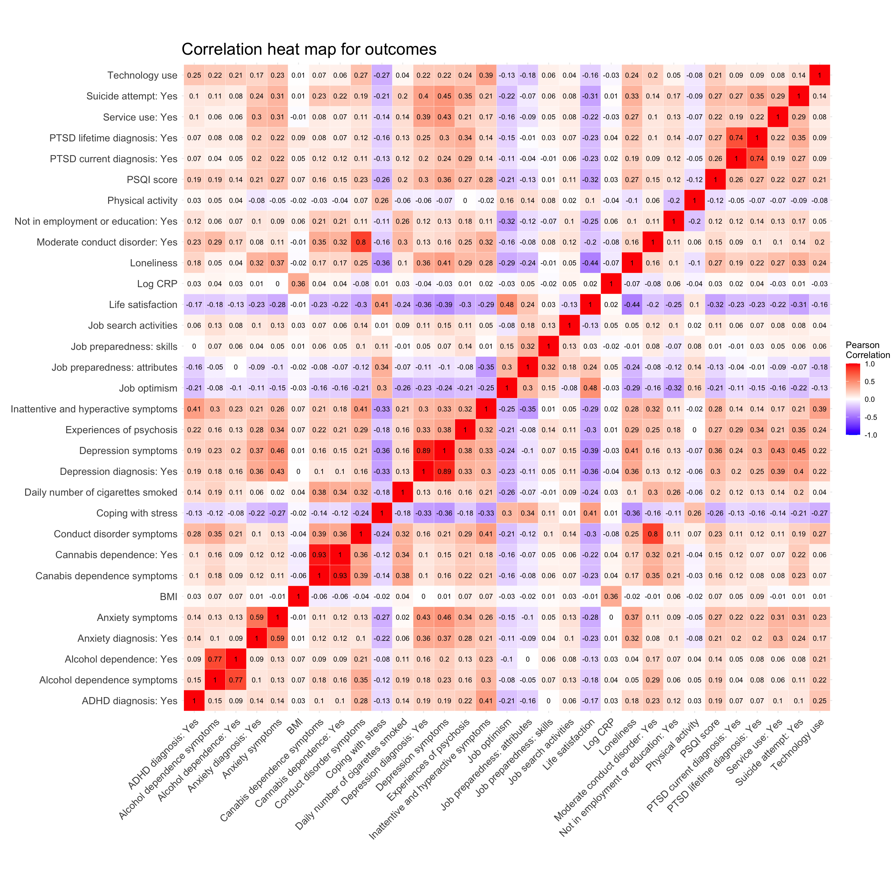
Association with outcome variables at age 18
Analysis Plan
Individual outcome regressions: single regressions are computed to see if the class can predict the the occurrence of each variable (variable ~ class). This is done through a loop. Odds Ratios (OR) and their confidence intervals are calculated for binary variables (logistic regression). Standardized Beta values are calculated for continuous variables (linear regression). Continuous and binary variables are plotted separately. Z scores are calculated for all continuous variables and all linear regressions are run using z scores.
A. Logistic regressions (binary variables): depression_diagnosis_12mo_18, anxiety_diagnosis_18, ADHD_diagnosis_18, conduct_disorder_moderate_18, alcohol_dependence_18, cannabis_dependence_18, PTSD_diagnosis_lifetime_18, PTSD_diagnosis_current_18,suicide_attempt_selfharm_18, service_use_18, not_in_employment_education_numeric_18. alcohol_abuse_18 removed as using alcohol_dependence_18 instead as it captures more disordered drinking.
B. Linear regressions (continuous variables): depression_current_scale_18, anxiety_current_scale_18, inattentive_hyperactive_symptoms_total_18, conduct_disorder_symptoms_18, alcohol_symptom_scale_18, cannabis_symptom_scale_18, cat_psychosis_experiences_scale_18, BMI_18, CRP_log_18, physical_activity_18, smoking_current_number_18, loneliness_18, life_satisfaction_18, technology_use_18, coping_with_stress_18, PSQI_global_score_18, job_preparedness_skills_18, job_preparedness_attributes_18, optimism_18, job_search_activities_count_18
C. Regressions rerun whilst controlling for antecedents (both continuous and binary are rerun): antecedents controlled for include: prosocial_behaviours_combined_05 + ADHD_combined_05 + internalising_combined_excl_sis_05 + maternal_personality_openness_05 + number_children_school_05
Preparation
Create z scores for all continuous variables
# create a scaled version of the continuous variables - z scores for all variables
scaled_continuous_data <- as.data.frame(scale(dat[outcome.dependent.linear], center = TRUE, scale = TRUE))

# rename variables to show that they are z scores
colnames(scaled_continuous_data) <- paste0("z_score.", colnames(scaled_continuous_data))

# combine the scaled data to the main dataset
dat <- cbind(dat, scaled_continuous_data)

#colnames(dat)
Posterior sensitivity analysis
The below few chunks are used to run the same analysis again in a reduced sample (only individuals who had a posterior probability of above 0.8 in all classes).
IMPORTANT: We created the current Rmd script to be able to use the same script to run the same analysis again in a reduced sample as a sensitivity analysis (only individuals who had a posterior probability of above 0.8 in all classes). When the variable “posterior.cut” is set to TRUE the following code will run for the data set that has those probability<0.8 dropped.
posterior.cut = FALSEif(posterior.cut == TRUE){
# create new variable only with those who have a probability higher than 0.8 for each class
dat <- dat %>%
mutate(class_renamed_cut =
factor(
case_when(
prob2 > 0.8 & class_renamed == "Increasing" ~ "Increasing",
prob3 > 0.8 & class_renamed == "Decreasing" ~ "Decreasing",
prob1 > 0.8 & class_renamed == "Low stable" ~ "Low stable"
),
ordered = FALSE))
library(nnet)
# check the biggest group in the class to be the reference group
table(dat$class_renamed_cut)
# relevel class_factor
dat <- dat %>%
mutate(
class_reordered_cut =
relevel(
class_renamed_cut,
ref = "Low stable",
first = TRUE, #levels in ref come first
collapse = "+", #String used when constructing names for combined factor levels
xlevels = TRUE #levels maintained even if not actually occurring
)
)
# check
table(dat$class_reordered_cut)
# create new data set with only these individuals
dat_prob_cut_out <- dat %>% filter(is.na(class_reordered_cut))
dat <- dat %>% filter(!is.na(class_reordered_cut))
# check
freq(dat$class_reordered)
}Statistics for posterior probability sensitivity analyses:
- Low stable: Dropped 42 people. Average probability = 0.66, minimum probability = 0.48.
- Increasing: Dropped 24 people. Average probability = 0.64, minimum probability = 0.49.
- Decreasing: Dropped 25 people. Average probability = 0.63, minimum probability = 0.51.
Posterior sensitivity N = 2141
if(posterior.cut == TRUE){
low.stable.cut.stats <- dat_prob_cut_out %>%
  filter(class_reordered == "Low stable") %>%
  descr(prob1)

increasing.cut.stats <- dat_prob_cut_out %>%
  filter(class_reordered == "Increasing") %>%
  descr(prob2)

decreasing.cut.stats <- dat_prob_cut_out %>%
  filter(class_reordered == "Decreasing") %>%
  descr(prob3)

low.stable.cut.stats
increasing.cut.stats
decreasing.cut.stats
}
Logistic regression
Loop
logistic.stats.outcome <- list() #create empty list to store the information in

for (i in 1:length(outcome.dependent.logistic))
{ cat(i)
  logistic.formula.outcome <- as.formula(sprintf("%s ~ class_reordered + sex + SES_ordered", outcome.dependent.logistic[i]))

  logistic.reg.outcome <- glm(logistic.formula.outcome, data = dat, family = "binomial")

  logistic.output.outcome.full <- huber.white.cluster.logistic(logistic.reg.outcome)

  logistic.output.outcome.full <- as.data.frame(logistic.output.outcome.full$coeftable)[-c(1,4:6),] %>% # delete sex and SES coefficients
    mutate(Class = c("Increasing", "Decreasing")) %>% # Create new formatted class variable
    dplyr::select(
      Class,
      OR = `exp(Est.)`,
      OR.conf.low = `2.5%`,
      OR.conf.high = `97.5%`,
      p.value = p)

  if (i < 11) {
    logistic.output.outcome.full <- logistic.output.outcome.full %>%
      mutate(block = "Mental health domain") %>%
      mutate(Variable = outcome.dependent.logistic.name.list[[i]])

  } else {
   logistic.output.outcome.full <- logistic.output.outcome.full %>%
      mutate(block = "Employment domain") %>%
      mutate(Variable = outcome.dependent.logistic.name.list[[i]])
  }

  logistic.output.outcome.full <- add.significance.variable(logistic.output.outcome.full)

  logistic.stats.outcome[[i]] <- logistic.output.outcome.full
}

# set the names of the list to match the variable names
names(logistic.stats.outcome) <- outcome.dependent.logistic
data.outcome.logistic <- create.dataset(logistic.stats.outcome, model = "logistic") Table
paper.table(data.outcome.logistic, model = "logistic")| Class | Variable | OR | 95% CI low | 95% CI high | p value | Domain |
|---|---|---|---|---|---|---|
| Increasing | Depression diagnosis | 1.32 | 0.81 | 2.15 | 0.26 | Mental health domain |
| Decreasing | Depression diagnosis | 1.57 | 1.00 | 2.45 | 0.05 | Mental health domain |
| Increasing | Anxiety diagnosis | 1.56 | 0.79 | 3.10 | 0.20 | Mental health domain |
| Decreasing | Anxiety diagnosis | 1.16 | 0.56 | 2.43 | 0.69 | Mental health domain |
| Increasing | ADHD diagnosis | 2.15 | 1.15 | 4.01 | 0.02 | Mental health domain |
| Decreasing | ADHD diagnosis | 1.78 | 0.95 | 3.32 | 0.07 | Mental health domain |
| Increasing | Moderate conduct disorder | 1.91 | 1.16 | 3.15 | 0.01 | Mental health domain |
| Decreasing | Moderate conduct disorder | 1.21 | 0.70 | 2.08 | 0.50 | Mental health domain |
| Increasing | Alcohol dependence | 0.73 | 0.36 | 1.45 | 0.36 | Mental health domain |
| Decreasing | Alcohol dependence | 0.84 | 0.46 | 1.55 | 0.58 | Mental health domain |
| Increasing | Cannabis dependence | 2.22 | 1.08 | 4.54 | 0.03 | Mental health domain |
| Decreasing | Cannabis dependence | 2.11 | 1.01 | 4.39 | 0.05 | Mental health domain |
| Increasing | PTSD lifetime diagnosis | 1.41 | 0.69 | 2.87 | 0.35 | Mental health domain |
| Decreasing | PTSD lifetime diagnosis | 1.12 | 0.54 | 2.34 | 0.75 | Mental health domain |
| Increasing | PTSD current diagnosis | 1.28 | 0.47 | 3.53 | 0.63 | Mental health domain |
| Decreasing | PTSD current diagnosis | 0.84 | 0.30 | 2.38 | 0.75 | Mental health domain |
| Increasing | Suicide attempt | 1.99 | 1.16 | 3.39 | 0.01 | Mental health domain |
| Decreasing | Suicide attempt | 1.69 | 1.02 | 2.79 | 0.04 | Mental health domain |
| Increasing | Service use | 1.91 | 1.10 | 3.32 | 0.02 | Mental health domain |
| Decreasing | Service use | 1.06 | 0.58 | 1.95 | 0.85 | Mental health domain |
| Increasing | Not in employment or education | 2.07 | 1.24 | 3.47 | 0.01 | Employment domain |
| Decreasing | Not in employment or education | 1.63 | 0.91 | 2.95 | 0.10 | Employment domain |
# mental health
data.outcome.logistic.mental <- order.variables(data.outcome.logistic, domain = "Mental health domain", model = "logistic")

# employment prospects
data.outcome.logistic.employ <- order.variables(data.outcome.logistic, domain = "Employment domain", model = "logistic")

# all
dat.logistic.ordered <- rbind(
  data.outcome.logistic.mental,
  data.outcome.logistic.employ
)
Plot
outcome.logistic.separate.plot <- ggplot(
  dat.logistic.ordered,
  aes(x = Variable,
      y = OR,
      ymin = OR.conf.low,
      ymax = OR.conf.high)
  ) +
  scale_shape_manual(values = c(21, 19)) +
  geom_pointrange(aes(shape = Significance), position = position_dodge(width = 0.7)) +
  facet_grid(Domain ~ Class, drop = TRUE, scales = "free_y", space = "free") +
  labs(y = "OR (95% CI)",
       x = "names",
       title = "Association between class membership and outcomes at age 18",
       color = "",
       shape = "") +
  scale_y_continuous(trans = scales::log10_trans(), breaks = c(0.2,0.4,0.6,0.8, 1, 1.5, 2, 3, 4)) +
  theme.outcome +
  geom_hline(linetype = "dashed", yintercept = 1) +
  coord_flip()

outcome.logistic.separate.plot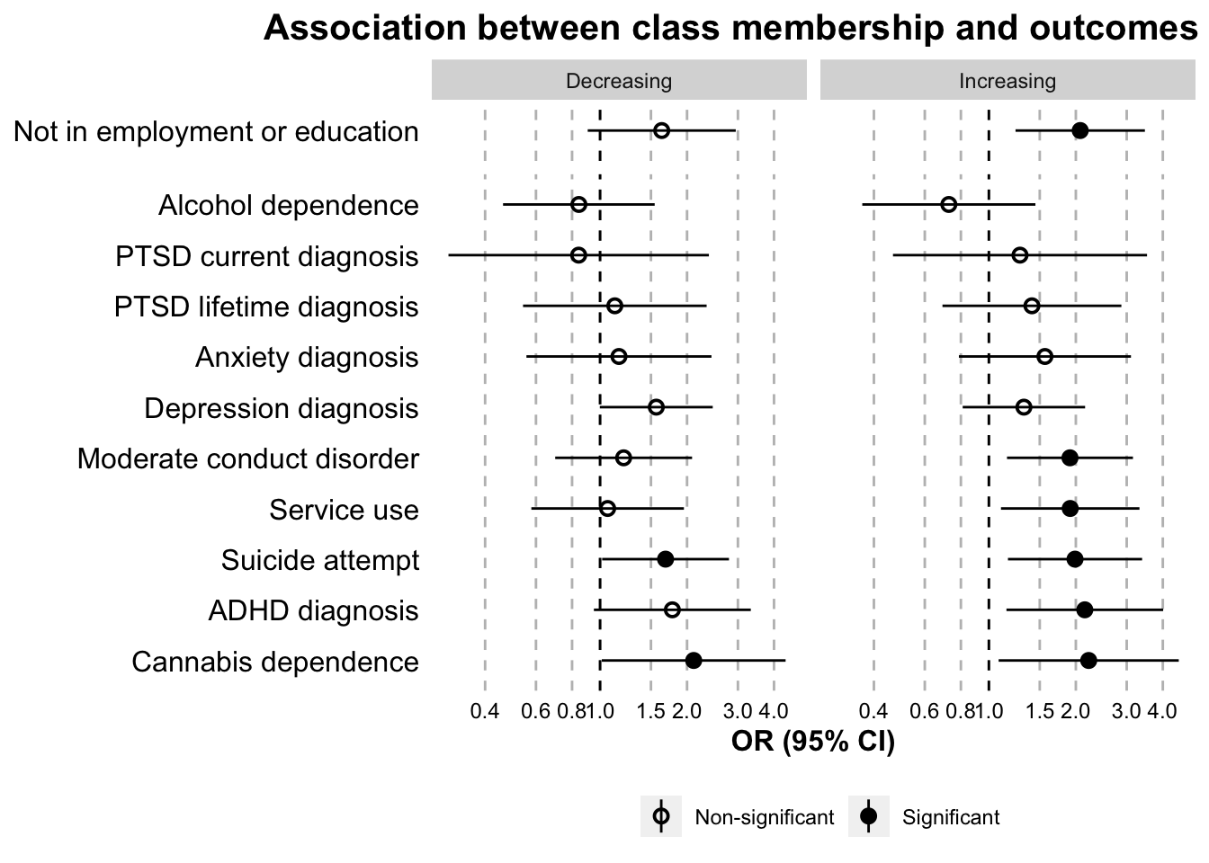
Linear regression
Using z-scores in all calculations.
Loop
linear.stats.outcome.zscore <- list() #create empty list to store the information in

for (i in 1:length(outcome.dependent.linear.zscore))
{ cat(i)
  linear.formula.outcome.zscore <- as.formula(sprintf("%s ~ class_reordered + sex + SES_ordered", outcome.dependent.linear.zscore[i]))

  linear.reg.outcome.zscore <- lm(linear.formula.outcome.zscore, data = dat)

  # robust standard error estimation - account for non-independence of twin sample
  linear.output.outcome.full.zscore <- huber.white.cluster.linear(linear.reg.outcome.zscore,
                                                                  rows.remove = -c(1,4:6))

  if (i < 8) {
    linear.output.outcome.full.zscore <- linear.output.outcome.full.zscore %>%
      mutate(block = "Mental health domain") %>%
      mutate(Variable = outcome.dependent.linear.name.list[[i]])
  } else if (i < 12 ) {
   linear.output.outcome.full.zscore <- linear.output.outcome.full.zscore %>%
      mutate(block = "Physical health domain") %>%
      mutate(Variable = outcome.dependent.linear.name.list[[i]])
  } else if (i < 17) {
    linear.output.outcome.full.zscore <- linear.output.outcome.full.zscore %>%
      mutate(block = "Coping and functioning domain") %>%
      mutate(Variable = outcome.dependent.linear.name.list[[i]])
  } else {
    linear.output.outcome.full.zscore <- linear.output.outcome.full.zscore %>%
      mutate(block = "Employment domain") %>%
      mutate(Variable = outcome.dependent.linear.name.list[[i]])
  }

  linear.output.outcome.full.zscore <- add.significance.variable(linear.output.outcome.full.zscore)

  linear.stats.outcome.zscore[[i]] <- linear.output.outcome.full.zscore
}
# set the names of the list to match the variable names
names(linear.stats.outcome.zscore) <- outcome.dependent.linear.zscore
data.outcome.linear.zscore <- create.dataset(linear.stats.outcome.zscore, model = "linear")Table
linear.table <- paper.table(data.outcome.linear.zscore, model = "linear")
linear.table | Class | Variable | Beta estimate | 95% CI low | 95% CI high | p value | Domain |
|---|---|---|---|---|---|---|
| Increasing | Depression symptoms | 0.20 | -0.02 | 0.43 | 0.08 | Mental health domain |
| Decreasing | Depression symptoms | 0.26 | 0.05 | 0.47 | 0.02 | Mental health domain |
| Increasing | Anxiety symptoms | 0.10 | -0.13 | 0.32 | 0.39 | Mental health domain |
| Decreasing | Anxiety symptoms | 0.07 | -0.14 | 0.27 | 0.52 | Mental health domain |
| Increasing | Inattentive and hyperactive symptoms | 0.57 | 0.36 | 0.79 | 0.00 | Mental health domain |
| Decreasing | Inattentive and hyperactive symptoms | -0.03 | -0.23 | 0.18 | 0.81 | Mental health domain |
| Increasing | Conduct disorder symptoms | 0.41 | 0.15 | 0.66 | 0.00 | Mental health domain |
| Decreasing | Conduct disorder symptoms | 0.06 | -0.16 | 0.28 | 0.60 | Mental health domain |
| Increasing | Alcohol dependence symptoms | -0.11 | -0.29 | 0.08 | 0.24 | Mental health domain |
| Decreasing | Alcohol dependence symptoms | 0.01 | -0.23 | 0.25 | 0.92 | Mental health domain |
| Increasing | Cannabis dependence symptoms | 0.23 | -0.03 | 0.49 | 0.09 | Mental health domain |
| Decreasing | Cannabis dependence symptoms | 0.30 | -0.01 | 0.62 | 0.06 | Mental health domain |
| Increasing | Experiences of psychosis | 0.35 | 0.09 | 0.60 | 0.01 | Mental health domain |
| Decreasing | Experiences of psychosis | 0.31 | 0.07 | 0.55 | 0.01 | Mental health domain |
| Increasing | BMI | 0.22 | -0.04 | 0.48 | 0.09 | Physical health domain |
| Decreasing | BMI | 0.03 | -0.15 | 0.21 | 0.74 | Physical health domain |
| Increasing | Log CRP | 0.07 | -0.16 | 0.30 | 0.55 | Physical health domain |
| Decreasing | Log CRP | 0.17 | -0.07 | 0.41 | 0.16 | Physical health domain |
| Increasing | Physical activity | -0.28 | -0.48 | -0.07 | 0.01 | Physical health domain |
| Decreasing | Physical activity | -0.43 | -0.60 | -0.25 | 0.00 | Physical health domain |
| Increasing | Daily number of cigarettes smoked | 0.46 | 0.08 | 0.84 | 0.02 | Physical health domain |
| Decreasing | Daily number of cigarettes smoked | 0.19 | -0.01 | 0.39 | 0.06 | Physical health domain |
| Increasing | Loneliness | 0.37 | 0.13 | 0.61 | 0.00 | Coping and functioning domain |
| Decreasing | Loneliness | 0.19 | -0.03 | 0.42 | 0.08 | Coping and functioning domain |
| Increasing | Life satisfaction | -0.29 | -0.52 | -0.06 | 0.01 | Coping and functioning domain |
| Decreasing | Life satisfaction | -0.20 | -0.42 | 0.02 | 0.08 | Coping and functioning domain |
| Increasing | Technology use | 0.24 | 0.02 | 0.46 | 0.03 | Coping and functioning domain |
| Decreasing | Technology use | 0.18 | -0.03 | 0.39 | 0.10 | Coping and functioning domain |
| Increasing | Coping with stress | -0.34 | -0.55 | -0.12 | 0.00 | Coping and functioning domain |
| Decreasing | Coping with stress | -0.08 | -0.27 | 0.12 | 0.45 | Coping and functioning domain |
| Increasing | PSQI score | 0.21 | 0.01 | 0.41 | 0.04 | Coping and functioning domain |
| Decreasing | PSQI score | 0.06 | -0.14 | 0.25 | 0.57 | Coping and functioning domain |
| Increasing | Job preparedness: skills | 0.01 | -0.23 | 0.24 | 0.96 | Employment domain |
| Decreasing | Job preparedness: skills | -0.03 | -0.24 | 0.18 | 0.76 | Employment domain |
| Increasing | Job preparedness: attributes | -0.37 | -0.62 | -0.13 | 0.00 | Employment domain |
| Decreasing | Job preparedness: attributes | -0.12 | -0.32 | 0.09 | 0.27 | Employment domain |
| Increasing | Job optimism | -0.58 | -0.80 | -0.36 | 0.00 | Employment domain |
| Decreasing | Job optimism | -0.27 | -0.47 | -0.07 | 0.01 | Employment domain |
| Increasing | Job search activities | -0.06 | -0.27 | 0.15 | 0.57 | Employment domain |
| Decreasing | Job search activities | 0.06 | -0.16 | 0.29 | 0.58 | Employment domain |
##Separate out data frames for each domain (this is done to order the plot later on by domain)

# mental health
data.outcome.linear.mental <- order.variables(data = data.outcome.linear.zscore, domain = "Mental health domain", model = "linear")
# physical health
data.outcome.linear.physical <- order.variables(data.outcome.linear.zscore, domain = "Physical health domain", model = "linear")
# coping and functioning
data.outcome.linear.coping <- order.variables(data.outcome.linear.zscore, domain = "Coping and functioning domain", model = "linear")
# employment prospects
data.outcome.linear.employ <- order.variables(data.outcome.linear.zscore, domain = "Employment domain", model = "linear")

# all
dat.linear.ordered <- rbind(
  data.outcome.linear.mental,
  data.outcome.linear.physical,
  data.outcome.linear.coping,
  data.outcome.linear.employ
)
Plot
outcome.linear.separate.plot.zscore <- ggplot(
  dat.linear.ordered,
  aes(x = Variable,
      y = estimate,
      ymin = conf.low,
      ymax = conf.high)
  ) +
  scale_fill_manual(values = c("black")) +
  scale_color_manual(values = c("black")) +
  scale_shape_manual(values = c(19)) +
  geom_pointrange(position = position_dodge(width = 0.7)) +
  facet_grid(Domain ~ Class,
             drop = TRUE,
             scales = "free_y",
             space = "free") +
  labs(y = "Standardised Beta Estimate (95% CI)",
       x = "names") +
  theme.outcome +
  theme(
    strip.text.x = element_text(
        size = 10, color = "black", face = "bold",
        ),
    strip.background = element_rect(
     color = "black", fill = "white", size = 0.5, linetype = "solid"
     ),
    plot.title = element_text(size = 12,face = "bold"),
        axis.title.x = element_text(size = 10, face = "bold"),
        axis.text.x = element_text(size = 8, colour = "black"),
        axis.text.y = element_text(size = 10)
  ) +
  geom_hline(linetype = "dashed", yintercept = 0) +
  scale_y_continuous(breaks=c(-1.5, -1, -0.75, -0.5, -0.25, 0, 0.25, 0.5, 0.75, 1, 1.5, 2)) +
  coord_flip()

outcome.linear.separate.plot.zscore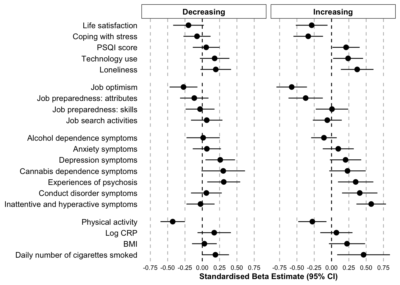
Controlling for significant antecedents
We have rerun all regression models while controlling for antecedents that remained significant in the full antecedent model. Antecedents that remained significant in the full antecedent model: child prosocial behaviours, child ADHD behaviours, child internalising behaviours, maternal personality openness, number of children in school. All regressions controlled for sex and SES.
Logistic regression: controlling for antecedents
Loop
logistic.stats.outcome.ant_control <- list() #create empty list to store the information in

for (i in 1:length(outcome.dependent.logistic))
{ cat(i)
  logistic.formula.outcome.ant_control <- as.formula(sprintf("%s ~ class_reordered + ADHD_combined_05 + internalising_combined_excl_sis_05 + prosocial_behaviours_combined_05 + maternal_personality_openness_05 + number_children_school_05 + sex + SES_ordered", outcome.dependent.logistic[i]))

  logistic.reg.outcome.ant_control <- glm(logistic.formula.outcome.ant_control, data = dat, family = "binomial")

  logistic.output.outcome.full.ant_control <- huber.white.cluster.logistic(logistic.reg.outcome.ant_control)

  logistic.output.outcome.full.ant_control <- as.data.frame(logistic.output.outcome.full.ant_control$coeftable)[-c(1,4:11),] %>% # delete sex and SES coefficients
    dplyr::mutate(Class = c("Increasing", "Decreasing")) %>% # Create new formatted class variable
    dplyr::select(
      Class,
      OR = `exp(Est.)`,
      OR.conf.low = `2.5%`,
      OR.conf.high = `97.5%`,
      p.value = p)

  if (i < 11) {
    logistic.output.outcome.full.ant_control <- logistic.output.outcome.full.ant_control %>%
      mutate(block = "Mental health domain") %>%
      mutate(Variable = outcome.dependent.logistic.name.list[[i]])
  } else {
   logistic.output.outcome.full.ant_control <- logistic.output.outcome.full.ant_control %>%
      mutate(block = "Employment domain") %>%
      mutate(Variable = outcome.dependent.logistic.name.list[[i]])
  }

  logistic.output.outcome.full.ant_control <- add.significance.variable(logistic.output.outcome.full.ant_control)

  logistic.stats.outcome.ant_control[[i]] <- logistic.output.outcome.full.ant_control
}
1234567891011
# set the names of the list to match the variable names
names(logistic.stats.outcome.ant_control) <- outcome.dependent.logistic
data.outcome.logistic.ant_control <- create.dataset(logistic.stats.outcome.ant_control, model = "logistic") Table
paper.table(data.outcome.logistic.ant_control, model = "logistic")| Class | Variable | OR | 95% CI low | 95% CI high | p value | Domain |
|---|---|---|---|---|---|---|
| Increasing | Depression diagnosis | 1.15 | 0.67 | 1.96 | 0.61 | Mental health domain |
| Decreasing | Depression diagnosis | 1.28 | 0.75 | 2.18 | 0.37 | Mental health domain |
| Increasing | Anxiety diagnosis | 1.18 | 0.52 | 2.67 | 0.69 | Mental health domain |
| Decreasing | Anxiety diagnosis | 1.09 | 0.50 | 2.38 | 0.83 | Mental health domain |
| Increasing | ADHD diagnosis | 1.19 | 0.60 | 2.36 | 0.61 | Mental health domain |
| Decreasing | ADHD diagnosis | 0.78 | 0.36 | 1.68 | 0.52 | Mental health domain |
| Increasing | Moderate conduct disorder | 1.56 | 0.90 | 2.69 | 0.11 | Mental health domain |
| Decreasing | Moderate conduct disorder | 0.90 | 0.47 | 1.73 | 0.75 | Mental health domain |
| Increasing | Alcohol dependence | 0.74 | 0.35 | 1.57 | 0.43 | Mental health domain |
| Decreasing | Alcohol dependence | 0.86 | 0.43 | 1.74 | 0.68 | Mental health domain |
| Increasing | Cannabis dependence | 1.76 | 0.77 | 4.04 | 0.18 | Mental health domain |
| Decreasing | Cannabis dependence | 1.34 | 0.59 | 3.03 | 0.48 | Mental health domain |
| Increasing | PTSD lifetime diagnosis | 1.32 | 0.60 | 2.92 | 0.49 | Mental health domain |
| Decreasing | PTSD lifetime diagnosis | 1.03 | 0.44 | 2.42 | 0.94 | Mental health domain |
| Increasing | PTSD current diagnosis | 1.14 | 0.35 | 3.73 | 0.83 | Mental health domain |
| Decreasing | PTSD current diagnosis | 0.75 | 0.22 | 2.56 | 0.65 | Mental health domain |
| Increasing | Suicide attempt | 1.77 | 1.00 | 3.14 | 0.05 | Mental health domain |
| Decreasing | Suicide attempt | 1.47 | 0.82 | 2.62 | 0.19 | Mental health domain |
| Increasing | Service use | 1.62 | 0.90 | 2.91 | 0.11 | Mental health domain |
| Decreasing | Service use | 0.74 | 0.37 | 1.51 | 0.41 | Mental health domain |
| Increasing | Not in employment or education | 1.35 | 0.77 | 2.38 | 0.30 | Employment domain |
| Decreasing | Not in employment or education | 0.75 | 0.38 | 1.48 | 0.41 | Employment domain |
Plot
outcome.logistic.separate.plot.ant_control <- ggplot(
  data.outcome.logistic.ant_control,
  aes(x = Variable,
      y = OR,
      ymin = OR.conf.low,
      ymax = OR.conf.high)
  ) +
  scale_shape_manual(values = c(21, 19)) +
  geom_pointrange(aes(shape = Significance), position = position_dodge(width = 0.7)) +
  facet_grid(Domain ~ Class, drop = TRUE, scales = "free_y", space = "free") +
  labs(y = "OR (95% CI)",
       x = "names",
       title = "Association betweenclass membership and outcomes at age 18",
       subtitle = paste("N(Total) = ", length(dat$sex),
                        "; N(Increasing) = ", sum(!is.na(dat$class_renamed[dat$class_renamed=="Increasing"])),
                        "; N(Decreasing) = ", sum(!is.na(dat$class_renamed[dat$class_renamed=="Decreasing"])), sep = ""),
       color = "",
       shape = ""
       ) +
  theme.outcome +
  geom_hline(linetype = "dashed", yintercept = 1) +
  scale_y_continuous(trans = scales::log10_trans(), breaks=c(0.2,0.4,0.6,0.8, 1, 1.5, 2, 2.5, 3, 4, 5)) +
  coord_flip()

outcome.logistic.separate.plot.ant_control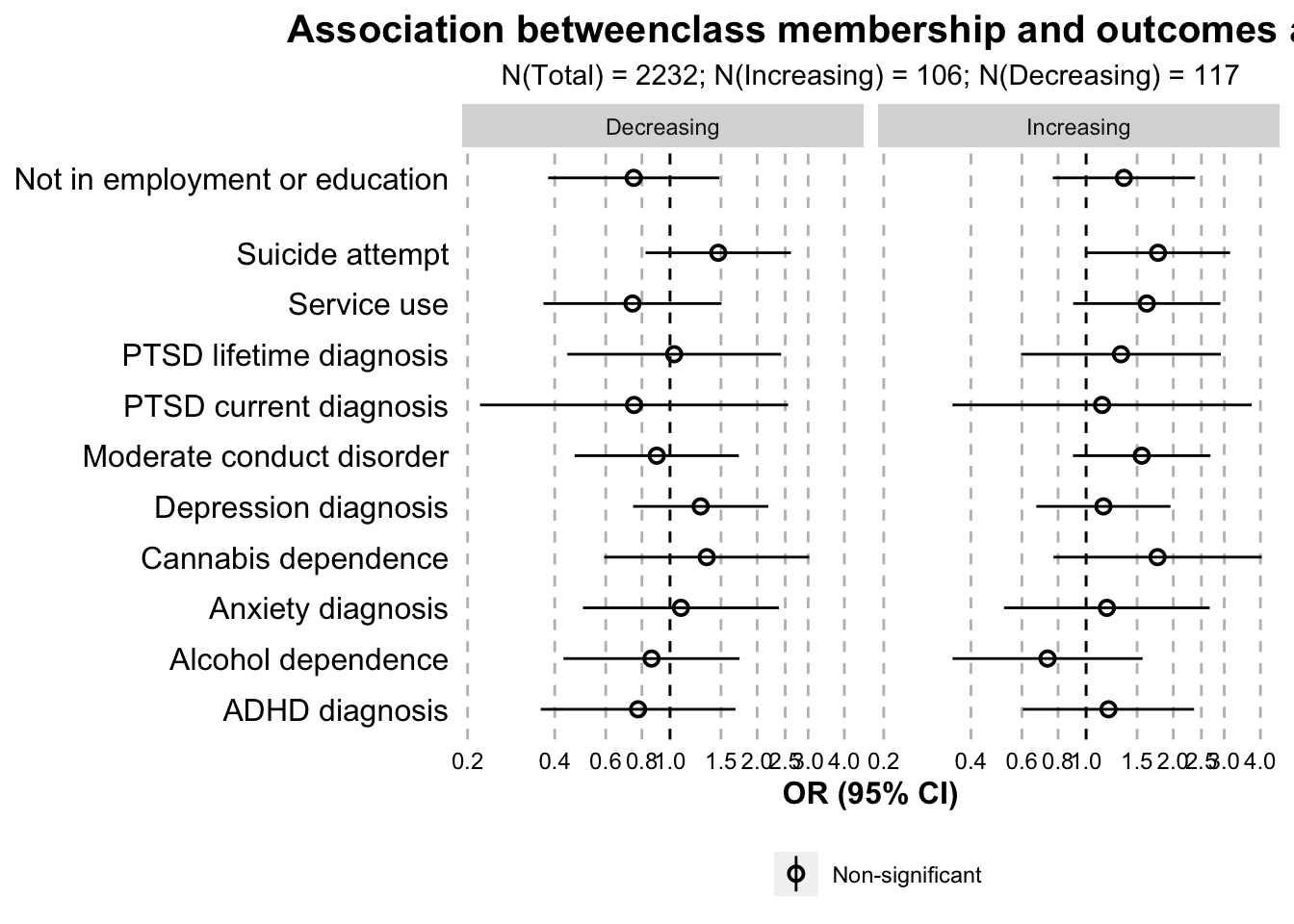
Linear regression: controlling for antecedents
Loop
linear.stats.outcome.zscore.ant_control <- list() #create empty list to store the information in

for (i in 1:length(outcome.dependent.linear.zscore))
{ cat(i)
  linear.formula.outcome.zscore.ant_control <- as.formula(sprintf("%s ~ class_reordered + prosocial_behaviours_combined_05 + ADHD_combined_05 + internalising_combined_excl_sis_05 + maternal_personality_openness_05 + number_children_school_05 + sex + SES_ordered", outcome.dependent.linear.zscore[i]))

  linear.reg.outcome.zscore.ant_control <- lm(linear.formula.outcome.zscore.ant_control, data = dat)

  # robust standard error estimation - account for non-independence of twin sample
  linear.output.outcome.full.zscore.ant_control <- huber.white.cluster.linear(regression.outcome = linear.reg.outcome.zscore.ant_control,
                                                                              rows.remove = -c(1,4:11))

  if (i < 8) {
    linear.output.outcome.full.zscore.ant_control <- linear.output.outcome.full.zscore.ant_control %>%
      mutate(block = "Mental health domain") %>%
      mutate(Variable = outcome.dependent.linear.name.list[[i]])
  } else if (i < 12 ) {
   linear.output.outcome.full.zscore.ant_control <- linear.output.outcome.full.zscore.ant_control %>%
      mutate(block = "Physical health domain") %>%
      mutate(Variable = outcome.dependent.linear.name.list[[i]])
  } else if (i < 17) {
    linear.output.outcome.full.zscore.ant_control <- linear.output.outcome.full.zscore.ant_control %>%
      mutate(block = "Coping and functioning domain") %>%
      mutate(Variable = outcome.dependent.linear.name.list[[i]])
  } else {
    linear.output.outcome.full.zscore.ant_control <- linear.output.outcome.full.zscore.ant_control %>%
      mutate(block = "Employment domain") %>%
      mutate(Variable = outcome.dependent.linear.name.list[[i]])
  }

  linear.output.outcome.full.zscore.ant_control <- add.significance.variable(linear.output.outcome.full.zscore.ant_control)

  linear.stats.outcome.zscore.ant_control[[i]] <- linear.output.outcome.full.zscore.ant_control
}
1234567891011121314151617181920
# set the names of the list to match the variable names
names(linear.stats.outcome.zscore.ant_control) <- outcome.dependent.linear.zscore
data.outcome.linear.zscore.ant_control <- create.dataset(linear.stats.outcome.zscore.ant_control, model = "linear")Table
linear.table.ant.control <- paper.table(data.outcome.linear.zscore.ant_control, model = "linear")
linear.table.ant.control| Class | Variable | Beta estimate | 95% CI low | 95% CI high | p value | Domain |
|---|---|---|---|---|---|---|
| Increasing | Depression symptoms | 0.14 | -0.10 | 0.38 | 0.26 | Mental health domain |
| Decreasing | Depression symptoms | 0.15 | -0.09 | 0.40 | 0.21 | Mental health domain |
| Increasing | Anxiety symptoms | -0.01 | -0.26 | 0.23 | 0.91 | Mental health domain |
| Decreasing | Anxiety symptoms | -0.07 | -0.31 | 0.17 | 0.55 | Mental health domain |
| Increasing | Inattentive and hyperactive symptoms | 0.35 | 0.12 | 0.58 | 0.00 | Mental health domain |
| Decreasing | Inattentive and hyperactive symptoms | -0.24 | -0.47 | -0.02 | 0.03 | Mental health domain |
| Increasing | Conduct disorder symptoms | 0.30 | 0.03 | 0.57 | 0.03 | Mental health domain |
| Decreasing | Conduct disorder symptoms | -0.10 | -0.33 | 0.14 | 0.42 | Mental health domain |
| Increasing | Alcohol dependence symptoms | -0.15 | -0.34 | 0.04 | 0.12 | Mental health domain |
| Decreasing | Alcohol dependence symptoms | -0.04 | -0.31 | 0.24 | 0.79 | Mental health domain |
| Increasing | Cannabis dependence symptoms | 0.14 | -0.15 | 0.43 | 0.34 | Mental health domain |
| Decreasing | Cannabis dependence symptoms | 0.17 | -0.15 | 0.49 | 0.30 | Mental health domain |
| Increasing | Experiences of psychosis | 0.20 | -0.07 | 0.47 | 0.14 | Mental health domain |
| Decreasing | Experiences of psychosis | 0.16 | -0.11 | 0.42 | 0.26 | Mental health domain |
| Increasing | BMI | 0.20 | -0.08 | 0.48 | 0.16 | Physical health domain |
| Decreasing | BMI | 0.05 | -0.17 | 0.26 | 0.67 | Physical health domain |
| Increasing | Log CRP | 0.08 | -0.17 | 0.33 | 0.52 | Physical health domain |
| Decreasing | Log CRP | 0.18 | -0.09 | 0.45 | 0.19 | Physical health domain |
| Increasing | Physical activity | -0.21 | -0.43 | 0.01 | 0.06 | Physical health domain |
| Decreasing | Physical activity | -0.27 | -0.48 | -0.06 | 0.01 | Physical health domain |
| Increasing | Daily number of cigarettes smoked | 0.37 | -0.03 | 0.77 | 0.07 | Physical health domain |
| Decreasing | Daily number of cigarettes smoked | -0.03 | -0.26 | 0.19 | 0.77 | Physical health domain |
| Increasing | Loneliness | 0.29 | 0.05 | 0.53 | 0.02 | Coping and functioning domain |
| Decreasing | Loneliness | 0.09 | -0.16 | 0.35 | 0.47 | Coping and functioning domain |
| Increasing | Life satisfaction | -0.17 | -0.41 | 0.07 | 0.17 | Coping and functioning domain |
| Decreasing | Life satisfaction | -0.04 | -0.29 | 0.22 | 0.77 | Coping and functioning domain |
| Increasing | Technology use | 0.13 | -0.10 | 0.35 | 0.26 | Coping and functioning domain |
| Decreasing | Technology use | 0.07 | -0.17 | 0.31 | 0.58 | Coping and functioning domain |
| Increasing | Coping with stress | -0.21 | -0.45 | 0.02 | 0.07 | Coping and functioning domain |
| Decreasing | Coping with stress | 0.10 | -0.12 | 0.33 | 0.36 | Coping and functioning domain |
| Increasing | PSQI score | 0.13 | -0.08 | 0.35 | 0.22 | Coping and functioning domain |
| Decreasing | PSQI score | -0.05 | -0.28 | 0.18 | 0.66 | Coping and functioning domain |
| Increasing | Job preparedness: skills | 0.13 | -0.12 | 0.37 | 0.32 | Employment domain |
| Decreasing | Job preparedness: skills | 0.15 | -0.09 | 0.39 | 0.22 | Employment domain |
| Increasing | Job preparedness: attributes | -0.19 | -0.46 | 0.07 | 0.15 | Employment domain |
| Decreasing | Job preparedness: attributes | 0.16 | -0.08 | 0.40 | 0.19 | Employment domain |
| Increasing | Job optimism | -0.40 | -0.64 | -0.16 | 0.00 | Employment domain |
| Decreasing | Job optimism | -0.03 | -0.26 | 0.19 | 0.78 | Employment domain |
| Increasing | Job search activities | -0.11 | -0.34 | 0.12 | 0.35 | Employment domain |
| Decreasing | Job search activities | 0.09 | -0.16 | 0.35 | 0.46 | Employment domain |
Plot
outcome.linear.separate.plot.zscore.ant_control <- ggplot(
  data.outcome.linear.zscore.ant_control,
  aes(x = Variable,
      y = estimate,
      ymin = conf.low,
      ymax = conf.high)
  ) +
  scale_shape_manual(values = c(21, 19)) +
  geom_pointrange(aes(shape = Significance), position = position_dodge(width = 0.7)) +
  facet_grid(Domain ~ Class, drop = TRUE, scales = "free_y", space = "free") +
  labs(y = "Standardised Estimate (95% CI)",
       x = "names",
       title = "Association between class membership and outcomes at age 18",
       subtitle = paste("N(Total) = ", length(dat$sex),
                        "; N(Increasing) = ", sum(!is.na(dat$class_renamed[dat$class_renamed=="Increasing"])),
                        "; N(Decreasing) = ", sum(!is.na(dat$class_renamed[dat$class_renamed=="Decreasing"])), sep = ""),
       color = "",
       shape = "") +
  theme.outcome +
  geom_hline(linetype = "dashed", yintercept = 0) +
 scale_y_continuous(breaks=c(-1.5, -1, -0.75, -0.5, -0.25, 0, 0.25, 0.5, 0.75, 1, 1.5, 2)) + # log10_trans() has been removed here
  coord_flip()

outcome.linear.separate.plot.zscore.ant_control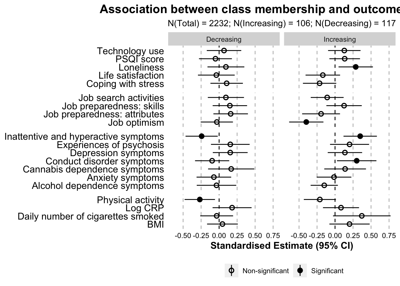
Work by Katherine N Thompson
katherine.n.thompson@kcl.ac.uk